6.3: Fine Structure of atomic Levels

Now let us use the same perturbation theory to analyze, also for the simplest case of a hydrogenlike atom/ion, the so-called fine structure of atomic levels - their degeneracy lifting even in the absence of external fields. Since the effective speed \(v\) of the electron motion in atoms is much smaller than the speed of light \(c\), the fine structure may be analyzed as a sum of two independent relativistic effects. To analyze the first of them, let us expand the well-known classical relativistic expression \({ }^{9}\) for the kinetic energy \(T=E-m c^{2}\) of a free particle with the rest mass \(m,{ }^{10}\) \[T=\left(m^{2} c^{4}+p^{2} c^{2}\right)^{1 / 2}-m c^{2} \equiv m c^{2}\left[\left(1+\frac{p^{2}}{m^{2} c^{2}}\right)^{1 / 2}-1\right],\] into the Taylor series with respect to the small ratio \((p / m c)^{2} \approx(v / c)^{2}\) : \[T=m c^{2}\left[1+\frac{1}{2}\left(\frac{p}{m c}\right)^{2}-\frac{1}{8}\left(\frac{p}{m c}\right)^{4}+\ldots-1\right] \equiv \frac{p^{2}}{2 m}-\frac{p^{4}}{8 m^{3} c^{2}}+\ldots\] and drop all the terms besides the two spelled-out terms. Of them, the first term is non-relativistic, while the second one represents the first relativistic correction to \(T\).

Following the correspondence principle, the quantum-mechanical problem in this approximation may be described by the perturbative Hamiltonian (1), whose unperturbed part (whose eigenstates and eigenenergies were discussed in \(\mathrm{Sec} .3 .5)\) is \[\hat{H}^{(0)}=\frac{\hat{p}^{2}}{2 m}+\hat{U}(r), \quad \hat{U}(r)=-\frac{C}{r},\] while the kinetic-relativistic perturbation
\[\hat{H}^{(1)}=-\frac{\hat{p}^{4}}{8 m^{3} c^{2}} \equiv-\frac{1}{2 m c^{2}}\left(\frac{\hat{p}^{2}}{2 m}\right)^{2}\] Using Eq. (46), we may rewrite the last formula as \[\hat{H}^{(1)}=-\frac{1}{2 m c^{2}}\left(\hat{H}^{(0)}-\hat{U}(r)\right)^{2},\] so that its matrix elements participating in the characteristic equation (25) for a given degenerate energy level (3.201), i.e. a given principal quantum number \(n\), are \[\left\langle n \operatorname{lm}\left|\hat{H}^{(1)}\right| n l^{\prime} m^{\prime}\right\rangle=-\frac{1}{2 m c^{2}}\left\langle n \operatorname{lm}\left|\left(\hat{H}^{(0)}-\hat{U}(r)\right)\left(\hat{H}^{(0)}-\hat{U}(r)\right)\right| n l^{\prime} m^{\prime}\right\rangle,\] where the bra- and ket-vectors describe the unperturbed eigenstates, whose eigenfunctions (in the coordinate representation) are given by Eq. (3.200): \(\psi_{n, l, m}=R_{n, l}(r) Y_{l}^{m}(\theta, \varphi)\).

It is straightforward (and hence left for the reader :-) to prove that all off-diagonal elements of the set (49) are equal to 0 . Thus we may use Eq. (27) for each set of the quantum numbers \(\{n, l, m\}\) : \[\begin{aligned} E_{n, l, m}^{(1)} & \equiv E_{n, l, m}-E_{n}^{(0)}=\left\langle n l m\left|\hat{H}^{(1)}\right| n l m\right\rangle=-\frac{1}{2 m c^{2}}\left\langle\left(\hat{H}^{(0)}-\hat{U}(r)\right)^{2}\right\rangle_{n, l, m} \\ &=-\frac{1}{2 m c^{2}}\left(E_{n}^{2}-2 E_{n}\langle\hat{U}\rangle_{n, l}+\left\langle\hat{U}^{2}\right\rangle_{n, l}\right)=-\frac{1}{2 m c^{2}}\left(\frac{E_{0}^{2}}{4 n^{4}}-\frac{E_{0}}{n^{2}} C\left\langle\frac{1}{r}\right\rangle_{n, l}+C^{2}\left\langle\frac{1}{r^{2}}\right\rangle_{n, l}\right) \end{aligned}\] where the index \(m\) has been dropped, because the radial wavefunctions \(\mathcal{R}_{n, l}(r)\), which affect these expectation values, do not depend on that quantum number. Now using Eqs. (3.191), (3.201) and the first two of Eqs. (3.211), we finally get \[E_{n, l}^{(1)}=-\frac{m C^{2}}{2 \hbar^{2} c^{2} n^{4}}\left(\frac{n}{l+1 / 2}-\frac{3}{4}\right) \equiv-\frac{2 E_{n}^{2}}{m c^{2}}\left(\frac{n}{l+1 / 2}-\frac{3}{4}\right)\] Let us discuss this result. First of all, its last form confirms that the correction (51) is indeed much smaller than the unperturbed energy \(E_{n}\) (and hence the perturbation theory is valid) if the latter is much smaller than the relativistic rest energy \(m c^{2}\) of the particle \(-\) as it is for the hydrogen atom. Next, since in the Bohr problem’s solution \(n \geq l+1\), the first fraction in the parentheses of Eq. (51) is always larger than 1 , and hence than \(3 / 4\), so that the kinetic relativistic correction to energy is negative for all \(n\) and \(l\). (Actually, this fact could be predicted already from Eq. (47), which shows that the perturbation’s Hamiltonian is a negatively defined form.) Finally, for a fixed principal number \(n\), the negative correction’s magnitude decreases with the growth of \(l\). This fact may be interpreted using the second of Eqs. (3.211): the larger is \(l\) (at fixed \(n\) ), the larger is the particle’s effective distance from the center, and hence the smaller is its effective velocity, i.e. the smaller is the magnitude of the quantum-mechanical average of the negative relativistic correction (47) to the kinetic energy.

The result (51) is valid for the Coulomb interaction \(U(r)=-C / r\) of any physical nature. However, if we speak specifically about hydrogen-like atoms/ions, there is also another relativistic correction to energy, due to the so-called spin-orbit interaction (alternatively called the "spin-orbit coupling"). Its physics may be understood from the following semi-quantitative classical reasoning: from the "the point of view" of an electron rotating about the nucleus at distance \(r\) with velocity \(\mathbf{v}\), it is the nucleus, of the electric charge \(Z e\), that rotates about the electron with the velocity \((-\mathbf{v})\) and hence the time period \(\tau=\) \(2 \pi r / v\). From the point of view of magnetostatics, such circular motion of the electric charge \(Q=Z e\), is equivalent to a circular dc electric current \(I=Q / T=(Z e)(v / 2 \pi r)\), which creates, at the electron’s location, i.e. in the center of the current loop, the magnetic field with the following magnitude: \({ }^{11}\) \[\mathscr{R}_{a}=\frac{\mu_{0}}{2 r} I=\frac{\mu_{0}}{2 r} \frac{Z e v}{2 \pi r} \equiv \frac{\mu_{0} Z e v}{4 \pi r^{2}} .\] The field’s direction \(\mathbf{n}\) is perpendicular to the apparent plane of the nucleus’ rotation (i.e. that of the real rotation of the electron), and hence its vector may be readily expressed via the similarly directed vector \(\mathbf{L}=m_{\mathrm{e}} v r \mathbf{n}\) of the electron’s angular (orbital) momentum: \[\mathscr{R}_{a}=\frac{\mu_{0} Z e v}{4 \pi r^{2}} \mathbf{n} \equiv \frac{\mu_{0} Z e}{4 \pi r^{3} m_{\mathrm{e}}} m_{\mathrm{e}} v r \mathbf{n} \equiv \frac{\mu_{0} Z e}{4 \pi r^{3} m_{\mathrm{e}}} \mathbf{L} \equiv \frac{Z e}{4 \pi \varepsilon_{0} r^{3} m_{\mathrm{e}} c^{2}} \mathbf{L},\] where the last step used the basic relation between the SI-unit constants: \(\mu_{0} \equiv 1 / c^{2} \varepsilon_{0}\).

A more careful (but still classical) analysis of the problem \({ }^{12}\) brings both good and bad news. The bad news is that the result (53) is wrong by the so-called Thomas factor of two even for the circular motion, because the electron moves with acceleration, and the reference frame bound to it cannot be inertial (as was implied in the above reasoning), so that the effective magnetic field felt by the electron is actually \[\mathscr{B}=\frac{Z e}{8 \pi \varepsilon_{0} r^{3} m_{\mathrm{e}} c^{2}} \mathbf{L} .\] The good news is that this result is valid not only for circular but an arbitrary orbital motion in the Coulomb field \(U(r)\). Hence from the discussion in Sec. \(4.1\) and Sec. \(4.4\) we may expect that the quantum-mechanical description of the interaction between this effective magnetic field and the electron’s spin moment (4.115) is given by the following perturbation Hamiltonian \({ }^{13}\) \[\hat{H}^{(1)}=-\hat{\mathbf{m}} \cdot \hat{\mathscr{B}}=-\gamma_{\mathrm{e}} \hat{\mathbf{S}} \cdot\left(\frac{Z e}{8 \pi \varepsilon_{0} r^{3} m_{\mathrm{e}} c^{2}} \hat{\mathbf{L}}\right) \equiv \frac{1}{2 m_{\mathrm{e}}^{2} c^{2}} \frac{Z e^{2}}{4 \pi \varepsilon_{0}} \frac{1}{r^{3}} \hat{\mathbf{S}} \cdot \hat{\mathbf{L}}\] where at spelling out the electron’s gyromagnetic ratio \(\gamma_{\mathrm{e}} \equiv-g_{\mathrm{e}} e / 2 m_{\mathrm{e}}\), the small correction to the value \(g_{\mathrm{e}}\) \(=2\) of the electron’s \(g\)-factor (see Sec. 4.4) is ignored, because Eq. (55) is already a small correction. This expectation is confirmed by the fully-relativistic Dirac theory, to be discussed in Sec. \(9.7\) below: it yields, for an arbitrary central potential \(U(r)\), the following spin-orbit coupling Hamiltonian: \[\hat{H}^{(1)}=\frac{1}{2 m_{\mathrm{e}}^{2} c^{2}} \frac{1}{r} \frac{d U(r)}{d r} \hat{\mathbf{S}} \cdot \hat{\mathbf{L}}\] For the Coulomb potential \(U(r)=-Z e^{2} / 4 \pi \varepsilon_{0} r\), this formula is reduced to Eq. (55).

As we already know from the discussion in Sec. 5.7, the angular factor of this Hamiltonian commutes with all the operators of the coupled-representation group (inside the blue line in Fig. 5.12): \(\hat{L}^{2}, \hat{S}^{2}, \hat{J}^{2}\), and \(\hat{J}_{z}\), and hence is diagonal in the coupled-representation basis with definite quantum numbers \(l, j\), and \(m_{j}\) (and of course \(s=1 / 2\) ). Hence, using Eq. (5.181) to rewrite Eq. (56) as \[\hat{H}^{(1)}=\frac{1}{2 m_{\mathrm{e}}^{2} c^{2}} \frac{Z e^{2}}{4 \pi \varepsilon_{0}} \frac{1}{r^{3}} \frac{1}{2}\left(\hat{J}^{2}-\hat{L}^{2}-\hat{S}^{2}\right),\] we may again use Eq. (27) for each set \(\left\{s, l, j, m_{j}\right\}\), with common \(n\) : \[E_{n, j, l}^{(1)}=\frac{1}{2 m_{\mathrm{e}}^{2} c^{2}} \frac{Z e^{2}}{4 \pi \varepsilon_{0}}\left\langle\frac{1}{r^{3}}\right\rangle_{n, l} \frac{1}{2}\left\langle\hat{J}^{2}-\hat{L}^{2}-\hat{S}^{2}\right\rangle_{j, s},\] where the indices irrelevant for each particular factor have been dropped. Now using the last of Eqs. (3.211), and similar expressions (5.169), (5.175), and (5.177) for eigenvalues of the involved operators, we get an explicit expression for the spin-orbit corrections \({ }^{14}\) \[E_{n, j, l}^{(1)}=\frac{1}{2 m_{\mathrm{e}}^{2} c^{2}} \frac{Z e^{2}}{4 \pi \varepsilon_{0}} \frac{\hbar^{2}}{2 r_{0}^{3}} \frac{j(j+1)-l(l+1)-3 / 4}{n^{3} l(l+1 / 2)(l+1)} \equiv \frac{E_{n}^{2}}{m_{\mathrm{e}} c^{2}} n \frac{j(j+1)-l(l+1)-3 / 4}{l(l+1 / 2)(l+1)},\] with \(l\) and \(j\) related by Eq. (5.189): \(j=l \pm 1 / 2\).

The last form of its result shows clearly that this correction has the same scale as the kinetic correction (51). \({ }^{15}\) In the \(1^{\text {st }}\) order of the perturbation theory, they may be just added (with \(m=m_{\mathrm{e}}\) ), giving a surprisingly simple formula for the net fine structure of the \(n^{\text {th }}\) energy level: \[E_{\text {fine }}^{(1)}=\frac{E_{n}^{2}}{2 m_{\mathrm{e}} c^{2}}\left(3-\frac{4 n}{j+1 / 2}\right) .\] This simplicity, as well as the independence of the result of the orbital quantum number \(l\), will become less surprising when (in Sec. 9.7) we see that this formula follows in one shot from the Dirac theory, in which the Bohr atom’s energy spectrum in numbered only with \(n\) and \(j\), but not \(l\). Let us recall that for an electron \((s=1 / 2)\), according to Eq. (5.189) with \(0 \leq l \leq n-1\), the quantum number \(j\) may take \(n\) positive half-integer values, from \(1 / 2\) to \(n-1 / 2\). Hence, Eq. (60) shows that the fine structure of the \(n^{\text {th }}\) Bohr’s energy level has \(n\) sub-levels - see Fig. 4 .

Please note that according to Eq. (5.175), each of these sub-levels is still \((2 j+1)\)-times degenerate in the quantum number \(m_{j} .\) This degeneracy is very natural, because in the absence of an external field the system is still isotropic. Moreover, on each fine-structure level (besides the highest one with \(j=n-1 / 2\) ), each of the \(m_{j}\)-states is doubly-degenerate in the orbital quantum number \(l=j \mp 1 / 2-\) see the labels of \(l\) in Fig. 4. (According to Eq. (5.190), each of these states, with fixed \(j\) and \(m_{j}\), may be represented as a linear combination of two states with adjacent values of \(l\), and hence different electron spin orientations, \(m_{s}=\pm 1 / 2\), weighed with the Clebsch-Gordan coefficients.)

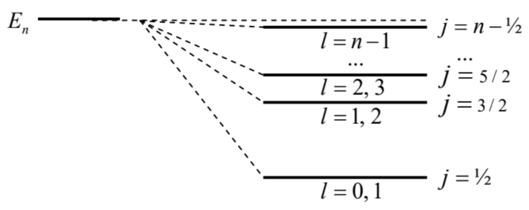Fig. 6.4. The fine structure of a hydrogen-like atom’s level.

These details aside, one may crudely say that the relativistic corrections combined make the total eigenenergy grow with \(l\), contributing to the effect already mentioned at our analysis of the periodic table of elements in Sec. 3.7. The relative scale of this increase may be scaled by the largest deviation from the unperturbed energy \(E_{n}\), reached for \(s\)-states (with \(l=0, j=1 / 2\) ): \[\frac{\left|E_{\max }^{(1)}\right|}{E_{n}}=\frac{E_{n}}{m_{\mathrm{e}} c^{2}}\left(2 n-\frac{3}{2}\right) \equiv\left(\frac{Z e^{2}}{4 \pi \varepsilon_{0} \hbar c}\right)^{2}\left(\frac{1}{n}-\frac{3}{4 n^{2}}\right) \equiv Z^{2} \alpha^{2}\left(\frac{1}{n}-\frac{3}{4 n^{2}}\right) .\] where \(\alpha\) is the fine-structure ("Sommerfeld’s") constant, \[\alpha \equiv \frac{e^{2}}{4 \pi \varepsilon_{0} \hbar c} \approx \frac{1}{137},\] (already mentioned in Sec. 4.4), which characterizes the relative strength (or rather weakness :-) of the electromagnetic effects in quantum mechanics - which in particular makes the perturbative quantum electrodynamics possible. \({ }^{16}\) These expressions show that the fine-structure splitting is a very small effect \(\left(\sim \alpha^{2} \sim 10^{-6}\right)\) for the hydrogen atom, but it rapidly grows (as \(Z^{2}\) ) with the nuclear charge (i.e. the atomic number) \(Z\), and becomes rather substantial for the heaviest stable atoms with \(Z \sim 10^{2}\).

---

\({ }^{9}\) See, e.g., EM Eq. (9.78) - or any undergraduate text on special relativity.

\({ }^{10}\) This fancy font is used, as in Secs. 3.5-3.8, to distinguish the mass \(m\) from the magnetic quantum number \(m\).

\({ }^{11}\) See, e.g., EM Sec. 5.1, in particular, Eq. (5.24). Note that such effective magnetic field is induced by any motion of electrons, in particular that in solids, leading to a variety of spin-orbit effects there - see, e.g., a concise review by R. Winkler et al., in B. Kramer (ed.), Advances in Solid State Physics \(\mathbf{4 1}, 211\) (2001).

\({ }^{12}\) It was carried out first by Llewellyn Thomas in 1926; for a simple review see, e.g., R. Harr and L. Curtis, \(A m\). J. Phys. \(\mathbf{5 5}, 1044\) (1987).

\({ }^{13}\) In the Gaussian units, Eq. (55) is valid without the factor \(4 \pi \varepsilon_{0}\) in the denominator; while Eq. (56), "as is".

\({ }^{14}\) The factor \(l\) in the denominator does not give a divergence at \(l=0\), because in this case \(j=s=1 / 2\), so that \(j(j+\) \(1)=3 / 4\), and the numerator turns into 0 as well. A careful analysis of this case (which may be found, e.g., in G. Woolgate, Elementary Atomic Structure, \(2^{\text {nd }}\) ed., Oxford, 1983), as well as the exact analysis of the hydrogen atom using the Dirac theory (see Sec. 9.7), show that Eq. (60), which does not include \(l\), is valid even in this case.

\({ }^{15}\) This is natural, because the magnetic interaction of charged particles is essentially a relativistic effect, of the same order \(\left(\sim v^{2} / c^{2}\right)\) as the kinetic correction (47) \(-\) see, e.g., EM Sec. 5.1, in particular Eq. (5.3).

\({ }^{16}\) The expression \(\alpha^{2}=E_{\mathrm{H}} / m_{\mathrm{e}} c^{2}\), where \(E_{\mathrm{H}}\) is the Hartree energy (1.13), i.e. the scale of energies \(E_{n}\), is also very revealing.