As a more involved example of the level degeneracy lifting by a perturbation, let us discuss the Stark effect 6 - the atomic level splitting by an external electric field. Let us study this effect, in the linear approximation, for a hydrogen-like atom/ion. Taking the direction of the external electric field E (which is practically always uniform on the atomic scale) for the z-axis, the perturbation may be represented by the following Hamiltonian: ˆH(1)=−Fˆz=−qEˆz=−qErcosθ.
(In the last form, the operator sign is dropped, because we will work in the coordinate representation.)
As you (should :-) remember, energy levels of a hydrogen-like atom/ion depend only on the principal quantum number n - see Eq. (3.201); hence all the states, besides the ground 1s state in which n=1 and l=m=0, have some orbital degeneracy, which grows rapidly with n. Let us consider the lowest degenerate level with n=2. Since, according to Eq. (3.203), 0≤l≤n−1, at this level the orbital quantum number l may equal either 0 (one 2s state, with m=0 ) or 1 (three 2p states, with m=0,±1 ). Due to this 4-fold degeneracy, H(1) is a 4×4 matrix with 16 elements: l=0⏞m=0l=1⏞m=0m=+1m=−1H(1)=(H11H12H13H14H21H22H23H24H31H32H33H34H41H42H43H44)m=0,m=0,m=0,mm=1.
However, there is no need to be scared. First, due to the Hermitian nature of the operator, only ten of these matrix elements (four diagonal and six off-diagonal ones) may be substantially different from each other. Moreover, due to a high symmetry of the problem, there are a lot of zeros even among these elements. Indeed, let us have a look at the angular components Yml of the corresponding wavefunctions, with l=0 and l=1, described by Eqs. (3.174)-(3.175). For the states with m=±1, the azimuthal parts of wavefunctions are proportional to exp{±iφ}; hence the off-diagonal elements H34 and H43 of the matrix (30), relating these functions, are proportional to ∮dΩY±1∗ˆH(1)Y∓1∝∫2π0dφ(e±iφ)∗(e∓iφ)=0.
The azimuthal-angle symmetry also kills the off-diagonal elements H13,H14,H23,H24 (and hence their complex conjugates H31,H41,H32, and H42 ), because they relate states with m=0 and m=±1, and hence are proportional to ∮dΩY0∗1ˆH(1)Y±11∝∫2π0dφe±iφ=0
For the diagonal matrix elements H33 and H44, corresponding to l=1 and m=±1, the azimuthal-angle integrals do not vanish, but since the corresponding spherical functions depend on the polar angle as sinθ, these elements are proportional to ∮dΩY±1∗1ˆH(1)Y±11∝∫π0sinθdθsinθcosθsinθ=∫+1−1cosθ(1−cos2θ)d(cosθ),
and hence are equal to zero - as any limit-symmetric integral of an odd function. Finally, for the states 2s and 2p with m=0, the diagonal elements H11 and H22 are also killed by the polar-angle integration: ∮dΩY0∗0ˆH(1)Y00∝∫π0sinθdθcosθ=∫1−1cosθd(cosθ)=0,∮dΩY1∗0ˆH(1)Y10∝∫π0sinθdθcos3θ=∫+1−1cos3θd(cosθ)=0.
Hence, the only non-zero elements of the matrix (30) are two off-diagonal elements H12 and H21, which relate two states with the same m=0, but different l={0,1}, because they are proportional to ∮dΩY0∗0cosθY01=√34π∫2π0dφ∫π0sinθdθcos2θ=1√3≠0.
What remains is to use Eqs. (3.209) for the radial parts of these functions to complete the calculation of those two matrix elements: H12=H21=−qE√3∫∞0r2drR2,0(r)rR2,1(r).
Due to the additive structure of the function R2,0(r), the integral falls into a sum of two table integrals, both of the type MA Eq. (6.7d), finally giving H12=H21=3qδr0,
where r0 is the spatial scale (3.192); for the hydrogen atom, it is just the Bohr radius rB - see Eq. (1.10).
Thus, the perturbation matrix (30) is reduced to H(1)=(03qEr0003qEr000000000000),
so that the condition (26) of self-consistency of the system (25), |−E(1)23qδr0003qδr0−E(1)20000−E(1)20000−E(1)2|=0
gives a very simple characteristic equation (E(1)2)2[(E(1)2)2−(3qEr0)2]=0.
with four roots: (E(1)2)1,2=0,(E(1)2)3,4=±3qEr0.
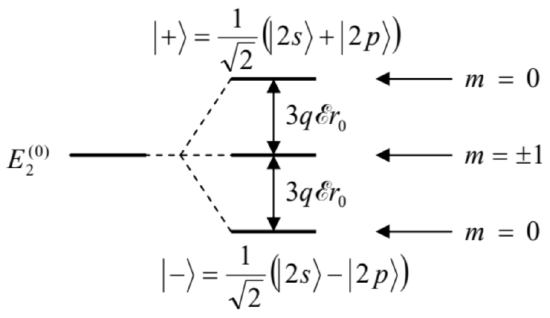
so that the degeneracy is only partly lifted - see the levels in Fig. 3. 7
Fig. 6.3. The linear Stark effect for the level n=2 of a hydrogen-like atom.
Generally, in order to understand the nature of states corresponding to these levels, we should return to Eq. (25) with each calculated value of E2(1), and find the corresponding expansion coefficients ⟨n′′(0)∣n′⟩ that describe the perturbed states. However, in our simple case, the outcome of this procedure is clear in advance. Indeed, since the states with {l=1,m=±1} are not affected by the perturbation at all (in the linear approximation in the electric field), their degeneracy is not lifted, and energy is not affected - see the middle line in Fig. 3. On the other hand, the partial perturbation matrix connecting the states 2s and 2p, i.e. the top left 2×2 part of the full matrix (39), is proportional to the Pauli matrix σx, and we already know the result of its diagonalization - see Eqs. (4.113)-(4.114). This means that the upper and lower split levels correspond to very simple linear combinations of the previously degenerate states with m=0, |±⟩=1√2(|2s⟩±|2p⟩).
Finally, let us estimate the magnitude of the linear Stark effect for a hydrogen atom. For a very high electric field of E=3×10⁶V/m,8|q|=e≈1.6×10−19C, and r0=rB≈0.5×10⁻¹⁰m, we get a level splitting of 3qδr0≈0.8×10⁻²²J≈0.5meV. This number is much lower than the unperturbed energy of the level, E2=−EH/(2×22)≈−3.4eV, so that the perturbative result is quite applicable. On the other hand, the calculated splitting is much larger than the resolution limit imposed by the line’s natural width (∼10−7E2, see Chapter 9), so that the effect is quite observable even in substantially lower electric fields. Note, however, that our simple results are quantitatively correct only when the Stark splitting (42) is much larger that the fine-structure splitting of the same level in the absence of the field- see the next section.
6 This effect was discovered experimentally in 1913 by Johannes Stark and independently by Antonio Lo Surdo, so it is sometimes (and more fairly) called the "Stark - Lo Surdo effect". Sometimes this name is used with the qualifier "dc" to distinguish it from the ac Stark effect - the energy level shift under the effect of an ac field - see Sec. 5 below.
7 The proportionality of this splitting to the small field is responsible for the qualifier "linear" in the name of this effect. If observable effects grow only as ε2 (see, e.g., Problem 9), the term quadratic Stark effect is used instead.
8 This value approximately corresponds to the threshold of electric breakdown in air at ambient conditions, due to the impact ionization. As a result, experiments with higher dc fields are rather difficult.