
8.2: Singlets, Triplets, and the Exchange Interaction


- Last updated
- Jan 29, 2022
- Save as PDF

( \newcommand{\kernel}{\mathrm{null}\,}\)
Now let us discuss possible approaches to quantitative analyses of identical particles, starting from a simple case of two spin-1/2 particles (say, electrons), whose explicit interaction with each other and the external world does not involve spin. The description of such a system may be based on factorable states with ket-vectors |α−⟩=|o12⟩⊗|s12⟩, with the orbital state vector |o12⟩ and the spin vector |s12⟩ belonging to different Hilbert spaces. It is frequently convenient to use the coordinate representation of such a state, sometimes called the spinor: ⟨r1,r2∣α−⟩=⟨r1,r2∣o12⟩⊗|s12⟩≡ψ(r1,r2)|s12⟩. Since the spin- 1/2 particles are fermions, the particle permutation has to change the sign:
ˆPψ(r1,r2)|s12⟩≡ψ(r2,r1)|s21⟩=−ψ(r1,r2)|s12⟩, of either the orbital factor or the spin factor.
In particular, in the case of symmetric orbital factor, ψ(r2,r1)=ψ(r1,r2), the spin factor has to obey the relation |s21⟩=−|s12⟩. Let us use the ordinary z-basis (where z, in the absence of an external magnetic field, is an arbitrary spatial axis) for both spins. In this basis, the ket-vector of any two spins- 1/2 may be represented as a linear combination of the following four basis vectors: |↑↑⟩,|↓↓⟩,|↑↓⟩, and |↓↑⟩. The first two kets evidently do not satisfy Eq. (16), and cannot participate in the state. Applying to the remaining kets the same argumentation as has resulted in Eq. (11), we get |s12⟩=|s−⟩≡1√2(|↑↓⟩−|↓↑⟩). Such an orbital-symmetric and spin-antisymmetric state is called the singlet.
The origin of this term becomes clear from the analysis of the opposite (orbital-antisymmetric and spin-symmetric) case: ψ(r2,r1)=−ψ(r1,r2),|s12⟩=|s21⟩. For the composition of such a symmetric spin state, the first two kets of Eq. (17) are completely acceptable (with arbitrary weights), and so is an entangled spin state that is the symmetric combination of the two last kets, similar to Eq. (10): |s+⟩≡1√2(|↑↓⟩+|↓↑⟩), so that the general spin state is a triplet: |s12⟩=c+|↑↑⟩+c−|↓↓⟩+c01√2(|↑↓⟩+|↓↑⟩). Note that any such state (with any values of the coefficients c satisfying the normalization condition), corresponds to the same orbital wavefunction and hence the same energy. However, each of these three states has a specific value of the z-component of the net spin - evidently equal to, respectively, +ℏ,−ℏ, and 0 . Because of this, even a small external magnetic field lifts their degeneracy, splitting the energy level in three; hence the term "triplet".
In the particular case when the particles do not interact at all, for example ˆH=ˆh1+ˆh2,ˆhk=ˆp2k2m+ˆu(rk), with k=1,2, the two-particle Schrödinger equation for the symmetrical orbital wavefunction (15) is obviously satisfied by the direct products, ψ(r1,r2)=ψn(r1)ψn′(r2), of single-particle eigenfunctions, with arbitrary sets n,n ’ of quantum numbers. For the particular but very important case n=n ’, this means that the eigenenergy of the (only acceptable) singlet state, 1√2(|↑↓⟩−|↓↑⟩)ψn(r1)ψn(r2), is just 2εn, where εn is the single-particle energy level. 9 In particular, for the ground state of the system, such singlet spin state gives the lowest energy Eg=2εg, while any triplet spin state (19) would require one of the particles to be in a different orbital state, i.e. in a state of higher energy, so that the total energy of the system would be also higher.
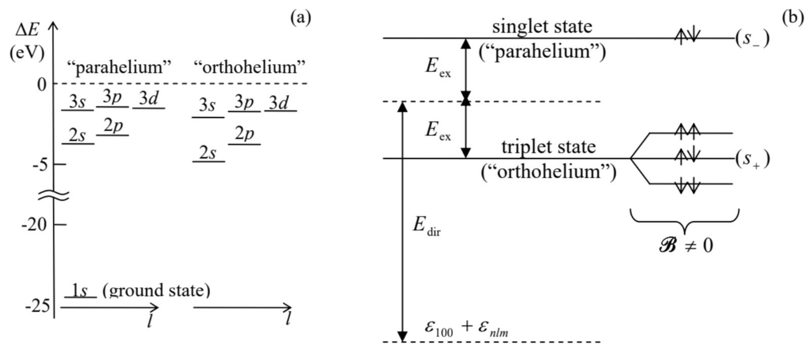
Now moving to the systems in which two indistinguishable spin- 1/2 particles do interact, let us consider, as their simplest but important 10 example, the lower energy states of a neutral atom 11 of helium - more exactly, 4He. Such an atom consists of a nucleus with two protons and two neutrons, with the total electric charge q=+2e, and two electrons "rotating" about the nucleus. Neglecting the small relativistic effects that were discussed in Sec. 6.3, the Hamiltonian describing the electron motion may be expressed as ˆH=ˆh1+ˆh2+ˆUint,ˆhk=ˆp2k2m−2e24πε0rk,ˆUint=e24πε0|r1−r2|. As with most problems of multiparticle quantum mechanics, the eigenvalue/eigenstate problem for this Hamiltonian does not have an exact analytical solution, so let us carry out its approximate analysis considering the electron-electron interaction Uint as a perturbation. As was discussed in Chapter 6 , we have to start with the " 0th -order" approximation in which the perturbation is ignored, so that the Hamiltonian is reduced to the sum (22). In this approximation, the ground state of the atom is the singlet (24), with the orbital factor ψg(r1,r2)=ψ100(r1)ψ100(r2), and energy 2εg. Here each factor ψ100(r) is the single-particle wavefunction of the ground (1s) state of the hydrogen-like atom with Z=2, with quantum numbers n=1,l=0, and m=0 - hence the wavefunctions’ indices. According to Eqs. (3.174) and (3.208), ψ100(r)=Y00(θ,φ)R1,0(r)=1√4π2r3/20e−r/r0, with r0=rBZ=rB2, and according to Eqs. (3.191) and (3.201), in this approximation the total ground state energy is E(0)g=2ε(0)g=2(−ε02n2)n=1,Z=2=2(−Z2EH2)Z=2=−4EH≈−109eV. This is still somewhat far (though not terribly far!) from the experimental value Eg≈−78.8eV− see the bottom level in Fig. 1a.
Making a minor (but very useful) detour from our main topic, let us note that we can get a much better agreement with experiment by calculating the electron interaction energy in the 1st order of the perturbation theory. Indeed, in application to our system, Eq. (6.14) reads E(1)g=⟨g|ˆUint|g⟩=∫d3r1∫d3r2ψ∗g(r1,r2)Uint(r1,r2)ψg(r1,r2). Plugging in Eqs. (25)-(27), we get E(1)g=(14π4r30)2∫d3r1∫d3r2e24πε0|r1−r2|exp{−2(r1+r2)r0}. As may be readily evaluated analytically (this exercise is left for the reader), this expression equals (5/4)EH, so that the corrected ground state energy, Eg≈E(0)g+E(1)g=(−4+5/4)EH=−74.8eV, is much closer to experiment.
There is still room here for a ready improvement, using the variational method discussed in Sec. 2.9. For our particular case of the 4He atom, we may try to use, as the trial state, the orbital wavefunction given by Eqs. (26)-(27), but with the atomic number Z considered as an adjustable parameter Zef <Z=2 rather than a fixed number. The physics behind this approach is that the electric charge density ρ(r)=−e|ψ(r)|2 of each electron forms a negatively charged "cloud" that reduces the effective charge of the nucleus, as seen by the other electron, to Zef e, with some Zef <2. As a result, the single-particle wavefunction spreads further in space (with the scale r0=rB/Zef>rB/Z ), while keeping its functional form (27) nearly intact. Since the kinetic energy T in the system’s Hamiltonian (25) is proportional to r0−2∝Zef2, while the potential energy is proportional to r0−1∝Zef1, we can write Eg(Zef )=(Zef 2)2⟨Tg⟩Z=2+Zef 2⟨Ug⟩Z=2. Now we can use the fact that according to Eq. (3.212), for any stationary state of a hydrogen-like atom (just as for the classical circular motion in the Coulomb potential), ⟨U⟩=2E, and hence ⟨T⟩=E− ⟨U⟩=−E. Using Eq. ( 30 ), and adding the correction (31) to the potential energy, we get Eg(Zef)=[4(Zef2)2+(−8+54)Zef2]EH. This expression allows an elementary calculation of the optimal value of Zef, and the corresponding minimum of the function Eg(Zef) : (Zef)opt=2(1−532)=1.6875,(Eg)min≈−2.85EH≈−77.5eV. Given the trial state’s crudeness, this number is in surprisingly good agreement with the experimental value cited above, with a difference of the order of 1%.
Now let us return to the main topic of this section - the effects of particle (in this case, electron) indistinguishability. As we have just seen, the ground-level energy of the helium atom is not affected directly by this fact, but the situation is different for its excited states - even the lowest ones. The reasonably good precision of the perturbation theory, which we have seen for the ground state, tells us that we can base our analysis of wavefunctions (ψe) of the lowest excited state orbitals, on products like ψ100(rk)ψnlm(rk′), with n>1. To satisfy the fermion permutation rule, Pj=−1, we have to take the orbital factor of the state in either the symmetric or the antisymmetric form: ψe(r1,r2)=1√2[ψ100(r1)ψnlm(r2)±ψnlm(r1)ψ100(r2)], with the proper total permutation asymmetry provided by the corresponding spin factor (18) or (21), so that the upper/lower sign in Eq. (35) corresponds to the singlet/triplet spin state. Let us calculate the expectation values of the total energy of the system in the first order of the perturbation theory. Plugging Eq. (35) into the 0th -order expression ⟨Ee⟩(0)=∫d3r1∫d3r2ψ∗e(r1,r2)(ˆh1+ˆh2)ψe(r1,r2), we get two groups of similar terms that differ only by the particle index. We can merge the terms of each pair by changing the notation as (r1→r,r2→r′) in one of them, and (r1→r′,r2→r) in the counterpart term. Using Eq. (25), and the mutual orthogonality of the wavefunctions ψ100(r) and ψnlm(r), we get the following result: ⟨Ee⟩(0)=∫ψ∗100(r)(−ℏ2∇2r2m−2e24πε0r)ψ100(r)d3r+∫ψ∗nlm(r′)(−ℏ2∇2r′2m−2e24πε0r′)ψnlm(r′)d3r′≡ε100+εnlm, with n>1 It may be interpreted as the sum of eigenenergies of two separate single particles, one in the ground state 100 , and another in the excited state nlm - although actually the electron states are entangled. Thus, in the 0th order of the perturbation theory, the electron entanglement does not affect their energy.
However, the potential energy of the system also includes the interaction term Uint , which does not allow such separation. Indeed, in the 1st approximation of the perturbation theory, the total energy Ee of the system may be expressed as ε100+εnlm+Eint (1), with E(1)int =⟨Uint ⟩=∫d3r1∫d3r2ψ∗e(r1,r2)Uint (r1,r2)ψe(r1,r2), Plugging Eq. (35) into this result, using the symmetry of the function Uint with respect to the particle number permutation, and the same particle coordinate re-numbering as above, we get E(1)int=Edir±Eex with the following, deceivingly similar expressions for the two components of this sum/difference: Edir≡∫d3r∫d3r′ψ∗100(r)ψ∗nlm(r′)Uint(r,r′)ψ100(r)ψnlm(r′),Eex≡∫d3r∫d3r′ψ∗100(r)ψ∗nlm(r′)Uint(r,r′)ψnlm(r)ψ100(r′). Since the single-particle orbitals can be always made real, both components are positive - or at least non-negative. However, their physics and magnitude are different. The integral (40), called the direct interaction energy, allows a simple semi-classical interpretation as the Coulomb energy of interacting electrons, each distributed in space with the electric charge density ρ(r)=−eψ∗(r)ψ(r):12 Edir=∫d3r∫d3r′ρ100(r)ρnmm(r′)4πε0|r−r′|≡∫ρ100(r)ϕnlm(r)d3r≡∫ρnm(r)ϕ100(r)d3r, where ϕ(r) are the electrostatic potentials created by the electron "charge clouds": 13 ϕ100(r)=14πε0∫d3r′ρ100(r′)|r−r′|,ϕnm(r)=14πε0∫d3r′ρnlm(r′)|r−r′|. However, the integral (41), called the exchange interaction energy, evades a classical interpretation, and (as it is clear from its derivation) is the direct corollary of electrons’ indistinguishability. The magnitude of Eex is also very much different from Edir because the function under the integral (41) disappears in the regions where the single-particle wavefunctions ψ100(r) and ψnlm(r) do not overlap. This is in full agreement with the discussion in Sec. 1: if two particles are identical but well separated, i.e. their wavefunctions do not overlap, the exchange interaction disappears, i.e. measurable effects of particle indistinguishability vanish. (In contrast, the integral (40) decreases with the growing electron separation only slowly, due to the long-range Coulomb interaction.)
Figure 1 b shows the structure of an excited energy level, with certain quantum numbers n>1,l, and m, given by Eqs. (39)-(41). The upper, so-called parahelium 14 level, with the energy Epara =(ε100+εnlm)+Edir +Eex >ε100+εnlm, corresponds to the symmetric orbital state and hence to the singlet spin state (18), while the lower, orthohelium level, with Eorth =(ε100+εnlm)+Edir −Eex <Epara , corresponds to the degenerate triplet spin state (21).
This degeneracy may be lifted by an external magnetic field, whose effect on the electron spins 15 is described by the following evident generalization of the Pauli Hamiltonian (4.163), ˆHfield =−ˆs1⋅B−ˆs2⋅B≡−ˆS⋅B, with γ=γe≡−eme≡−2μBℏ, where ˆS≡ˆs1+ˆs2, is the operator of the (vector) sum of the system of two spins. 16 To analyze this effect, we need first to make one more detour, to address the general issue of spin addition. The main rule 17 here is that in a full analogy with the net spin of a single particle, defined by Eq. (5.170), the net spin operator (47) of any system of two spins, and its component ˆSz along the (arbitrarily selected) z-axis, obey the same commutation relations (5.168) as the component operators, and hence have the properties similar to those expressed by Eqs. (5.169) and (5.175): ˆS2|S,MS⟩=ℏ2S(S+1)|S,MS⟩,ˆSz|S,MS⟩=ℏMS|S,MS⟩, with −S≤MS≤+S, where the ket vectors correspond to the coupled basis of joint eigenstates of the operators of S2 and Sz (but not necessarily all component operators - see again the Venn shown in Fig. 5.12 and its discussion, with the replacements S,L→s1,2 and J→S ). Repeating the discussion of Sec. 5.7 with these replacements, we see that in both coupled and uncoupled bases, the net magnetic number MS is simply expressed via those of the components MS=(ms)1+(ms)2. However, the net spin quantum number S (in contrast to the Nature-given spins s1,2 of its elementary components) is not universally definite, and we may immediately say only that it has to obey the following analog of the relation |l−s|≤j≤(l+s) discussed in Sec. 5.7: |s1−s2|≤S≤s1+s2. What exactly S is (within these limits), depends on the spin state of the system.
For the simplest case of two spin-1/2 components, each with s=1/2 and ms=±1/2, Eq. (49) gives three possible values of MS, equal to 0 and ±1, while Eq. (50) limits the possible values of S to just either 0 or 1 . Using the last of Eqs. (48), we see that the possible combinations of the quantum numbers are {S=0,MS=0, and {S=1,MS=0,±1. It is virtually evident that the singlet spin state s−belongs to the first class, while the simple (separable) triplet states ↑↑ and ↓↓ belong to the second class, with MS=+1 and MS=−1, respectively. However, for the entangled triplet state s+, evidently with MS=0, the value of S is less obvious. Perhaps the easiest way to recover it 18 to use the "rectangular diagram", similar to that shown in Fig. 5.14, but redrawn for our case of two spins, i.e., with the replacements ml→(ms)1=±1/2,ms→(ms)2=±1/2− see Fig. 2 .
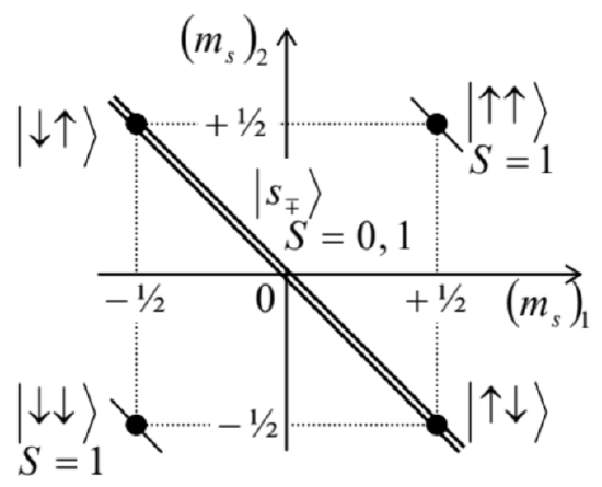
Just as at the addition of various angular momenta of a single particle, the top-right and bottomleft corners of this diagram correspond to the factorable triplet states ↑↑ and ↓↓, which participate in both the uncoupled-representation and coupled-representation bases, and have the largest value of S, i.e. 1. However, the entangled states s±, which are linear combinations of the uncoupled-representation states ↑↓ and ↓↑, cannot have the same value of S, so that for the triplet state S+,S has to take the value different from that (0) of the singlet state, i.e. 1. With that, the first of Eqs. (48) gives the following expectation values for the square of the net spin operator: ⟨S2⟩={2ℏ2, for each triplet state, 0, for the singlet state. Note that for the entangled triplet state s+, whose ket-vector (20) is a linear superposition of two kets of states with opposite spins, this result is highly counter-intuitive, and shows how careful we should be interpreting entangled quantum states. (As will be discussed in Chapter 10, the entanglement brings even more surprises for quantum measurements.)
Now we may return to the particular issue of the magnetic field effect on the triplet state of the 4He atom. Directing the z-axis along the field, we may reduce Eq. (46) to ˆHfield =−γeˆSzB≡2μBRˆSzℏ. Since all three triplet states (21) are eigenstates, in particular, of the operator ˆSz, and hence of the Hamiltonian (53), we may use the second of Eqs. (48) to calculate their energy change simply as ΔEfield =2μBBMS=2μBB×{+1, for the factorable triplet state ↑↑,0, for the entangled triplet state s+,−1, for the factorable triplet state ↓↓. This splitting of the "orthohelium" level is schematically shown in Fig. 1 b.19
9 In this chapter, I try to use lower-case letters for all single-particle observables (in particular, ε for their energies), in order to distinguish them as clearly as possible from the system’s observables (including the total energy E of the system), which are typeset in capital letters.
10 Indeed, helium makes up more than 20% of all "ordinary" matter of our Universe.
11 Note that the positive ion He+1 of this atom, with just one electron, is fully described by the hydrogen-like atom theory with Z=2, whose ground-state energy, according to Eq. (3.191), is −Z2EH/2=−2EH≈−55.4eV.
12 See, e.g., EM Sec. 1.3, in particular Eq. (1.54).
13 Note that the result for Edir correctly reflects the basic fact that a charged particle does not interact with itself, even if its wavefunction is quantum-mechanically spread over a finite space volume. Unfortunately, this is not true for some popular approximate theories of multiparticle systems - see Sec. 4 below.
14 This terminology reflects the historic fact that the observation of two different hydrogen-like spectra, corresponding to the opposite signs in Eq. (39), was first taken as evidence for two different species of 4He, which were called, respectively, the "orthohelium" and the "parahelium".
15 As we know from Sec. 6.4, the field also affects the orbital motion of the electrons, so that the simple analysis based on Eq. (46) is strictly valid only for the s excited state (l=0, and hence m=0). However, the orbital effects of a weak magnetic field do not affect the triplet level splitting we are analyzing now.
16 Note that similarly to Eqs. (22) and (25), here the uppercase notation of the component spins is replaced with their lowercase notation, to avoid any possibility of their confusion with the total spin of the system.
17 Since we already know that the spin of a particle is physically nothing more than a (specific) part of its angular momentum, the similarity of the properties (48) of the sum (47) of spins of different particles to those of the sum (5.170) of different spin components of the same particle it very natural, but still has to be considered as a new fact - confirmed by a vast body of experimental data.
18 Another, a bit longer but perhaps a more prudent way is to directly calculate the expectation values of ˆS2 for the states S±, and then find S by comparing the results with the first of Eqs. (48); it is highly recommended to the reader as a useful exercise.
19 It is interesting that another very important two-electron system, the hydrogen (H2) molecule, which was briefly discussed in Sec. 2.6, also has two similarly named forms, parahydrogen and orthohydrogen. However, their difference is due to two possible (respectively, singlet and triplet) states of the system of two spins of the two hydrogen nuclei - protons, which are also spin-1/2 particles. The resulting energy of the parahydrogen is lower than that of the orthohydrogen by only ∼45meV per molecule - the difference comparable with kBT at room temperature (∼26meV). As a result, at the ambient conditions, the equilibrium ratio of these two spin isomers is close to 3:1. Curiously, the theoretical prediction of this minor effect by W. Heisenberg (together with F. Hund) in 1927 was cited in his 1932 Nobel Prize award as the most noteworthy application of quantum theory.