8.5: Quantum Computation and Cryptography

Now I have to review the emerging fields of quantum computation and encryption. (Since these fields are much related, they are often referred to under the common title of "quantum information science", though this term is somewhat misleading, de-emphasizing physical aspects of the topic.) These fields are currently the subject of intensive research and development efforts, which has already brought, besides an enormous body of hype, some results of general importance. My coverage, by necessity short, will focus on these results, referring the reader interested in details to special literature. \({ }^{42}\) Because of the very active stage of the fields, I will also provide quite a few references to recent publications, making the style of this section closer to a brief literature review than to a textbook’s section.

Presently, most work on quantum computation and encryption is based on systems of spatially separated (and hence distinguishable) two-level systems - in this context, universally called qubits. \({ }^{43}\) Due to this distinguishability, the issues that were the focus of the first sections of this chapter, including the second quantization approach, are irrelevant here. On the other hand, systems of qubits have some interesting properties that have not been discussed in this course yet.

First of all, a system of \(N>>1\) qubits may contain much more information than the same number of \(N\) classical bits. Indeed, according to the discussions in Chapter 4 and Sec. 5.1, an arbitrary pure state of a single qubit may be represented by its ket vector (4.37) - see also Eq. (5.1): \[|\alpha\rangle_{N=1}=\alpha_{1}\left|u_{1}\right\rangle+\alpha_{2}\left|u_{2}\right\rangle,\] where \(\left\{u_{j}\right\}\) is any orthonormal two-state basis. It is natural and common to employ, as \(u_{j}\), the eigenstates \(a_{j}\) of the observable \(A\) that is eventually measured in the particular physical implementation of the qubit - say, a certain Cartesian component of spin- \(-1 / 2\). It is also common to write the kets of these base states as \(|0\rangle\) and \(|1\rangle\), so that Eq. (132) takes the form

\[\ \alpha\rangle_{N=1}=a_{0}|0\rangle+a_{1}|1\rangle \equiv \sum_{j=0,1} a_{j}|j\rangle\] (Here, and in the balance of this section, the letter \(j\) is used to denote an integer equal to either 0 or 1 .) According to this relation, any state \(\alpha\) of a qubit is completely defined by two complex \(c\)-numbers \(a_{j}\), i.e. by 4 real numbers. Moreover, due to the normalization condition \(\left|a_{1}\right|^{2}+\left|a_{2}\right|^{2}=1\), we need just 3 independent real numbers - say, the Bloch sphere coordinates \(\theta\) and \(\varphi\) (see Fig. 5.3), plus the common phase \(\gamma\), which becomes important only when we consider coherent states of a several-qubit system.

This is a good time to note that a qubit is very much different from any classical bistable system used to store single bits of information - such as two possible voltage states of the usual SRAM cell (essentially, a positive-feedback loop of two transistor-based inverters). Namely, the stationary states of a classical bistable system, due to its nonlinearity, are stable with respect to small perturbations, so that they may be very robust to unintentional interaction with their environment. In contrast, the qubit’s state may be disturbed (i.e. its representation point on the Bloch sphere shifted) by even minor perturbations, because it does not have such an internal state stabilization mechanism. \({ }^{44}\) Due to this reason, qubit-based systems are rather vulnerable to environment-induced drifts, including the dephasing and relaxation discussed in the previous chapter, creating major experimental challenges - see below.

Now, if we have a system of 2 qubits, the vectors of its arbitrary pure state may be represented as a sum of \(2^{2}=4\) terms, \({ }^{45}\) \[|\alpha\rangle_{N=2}=a_{00}|00\rangle+a_{01}|01\rangle+a_{10}|10\rangle+a_{11}|11\rangle \equiv \sum_{j_{1}, j_{2}=0,1} a_{j_{1} j_{2}}\left|j_{1} j_{2}\right\rangle\] with four complex coefficients, i.e. eight real numbers, subject to just one normalization condition, which follows from the requirement \(\langle\alpha \mid \alpha\rangle=1\) : \[\sum_{j_{1,2}=0,1}\left|a_{j_{1} j_{2}}\right|^{2}=1 .\] The evident generalization of Eqs. (133)-(134) to an arbitrary pure state of an \(N\)-qubit system is a sum of \(2^{N}\) terms: \[|\alpha\rangle_{N}=\sum_{j_{1}, j_{2}, \ldots j_{N}=0,1} a_{j_{1} j_{2} \ldots j_{N}}\left|j_{1} j_{2} \ldots j_{N}\right\rangle,\] including all possible combinations of 0 s and 1 s for indices \(j\), so that the state is fully described by \(2^{N}\) complex numbers, i.e. \(2 \cdot 2^{N} \equiv 2^{N+1}\) real numbers, with only one constraint, similar to Eq. (135), imposed by the normalization condition. Let me emphasize that this exponential growth of the information contents would not be possible without the qubit state entanglement. Indeed, in the particular case when qubit states are not entangled, i.e. are factorable:

\[\ \alpha\rangle_{N}=\left|\alpha_{1}\right\rangle\left|\alpha_{2}\right\rangle \ldots\left|\alpha_{N}\right\rangle\] where each \(\left|\alpha_{n}\right\rangle\) is described by an equality similar to Eq. (133) with its individual expansion coefficients, the system state description requires only \(3 N-1\) real numbers - e.g., \(N\) sets \(\{\theta, \varphi, \gamma\}\) less one common phase.

However, it would be wrong to project this exponential growth of information contents directly on the capabilities of quantum computation, because this process has to include the output information readout, i.e. qubit state measurements. Due to the fundamental intrinsic uncertainty of quantum systems, the measurement of a single qubit even in a pure state (133) generally may give either of two results, with probabilities \(W_{0}=\left|a_{0}\right|^{2}\) and \(W_{1}=\left|a_{1}\right|^{2}\). To comply with the general notion of computation, any quantum computer has to provide certain (or virtually certain) results, and hence the probabilities \(W_{j}\) have to be very close to either 0 or 1 , so that before the measurement, each measured qubit has to be in a basis state - either 0 or 1 . This means that the computational system with \(N\) output qubits, just before the final readout, has to be in one of the factorable states \[|\alpha\rangle_{N}=\left|j_{1}\right\rangle\left|j_{2}\right\rangle \ldots\left|j_{N}\right\rangle \equiv\left|j_{1} j_{2} \ldots j_{N}\right\rangle,\] which is a very small subset even of the set of all unentangled states (137), and whose maximum information contents is just \(N\) classical bits.

Now the reader may start thinking that this constraint strips quantum computations of any advantages over their classical counterparts, but such a view is also superficial. To show that, let us consider the scheme of the most actively explored type of quantum computation, shown in Fig. \(3 .{ }^{46}\)

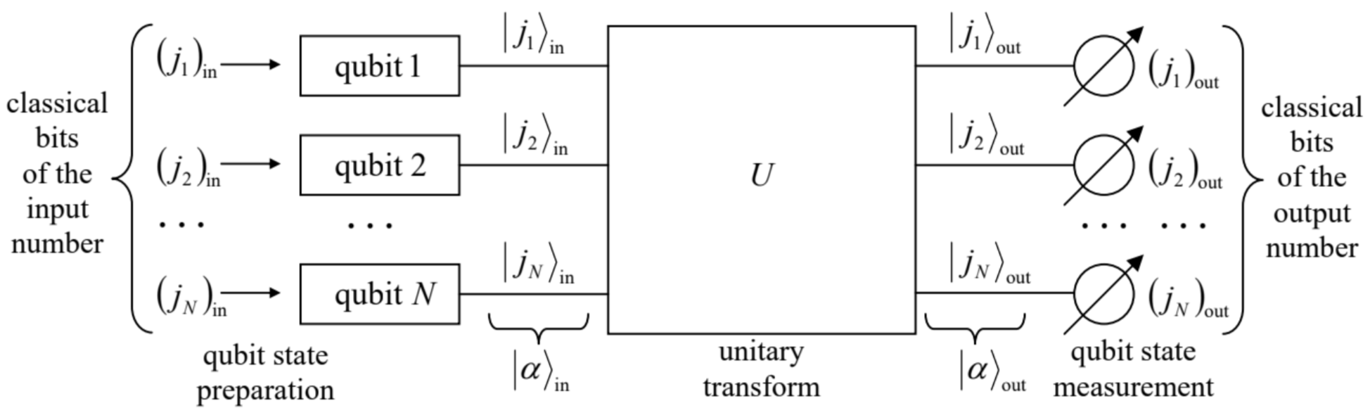Fig. 8.3. The baseline scheme of quantum computation.

Here each horizontal line (sometimes called a "wire" 47 ) corresponds to a single qubit, tracing its time evolution in the same direction as at the usual time function plots: from left to right. This means that the left column \(|\alpha\rangle_{\text {in }}\) of ket-vectors describes the initial state of the qubits, \({ }^{48}\) while the right column \(|\alpha\rangle_{\text {out }}\) describes their final (but pre-measurement) state. The box labeled \(U\) represents the qubit evolution in time due to their specially arranged interactions between each other and/or external drive "forces". Besides these forces, during this evolution the system is supposed to be ideally isolated from the dephasing and energy-dissipating environment, so that the process may be described by a unitary operator defined in the \(2^{N}\)-dimensional Hilbert space of \(N\) qubits: \[|\alpha\rangle_{\text {out }}=\hat{U}|\alpha\rangle_{\text {in }}\] With the condition that the input and output states have the simple form (138), this equality reads \[\left|\left(j_{1}\right)_{\text {out }}\left(j_{2}\right)_{\text {out }} \ldots\left(j_{N}\right)_{\text {out }}\right\rangle=\hat{U}\left|\left(j_{1}\right)_{\text {in }}\left(j_{2}\right)_{\text {in }} \ldots\left(j_{N}\right)_{\text {in }}\right\rangle .\] The art of quantum computer design consists of selecting such unitary operators \(\hat{U}\) that would:

• satisfy Eq. (140),
• be physically implementable, and
• enable substantial performance advantages of the quantum computation over its classical counterparts with similar functionality, at least for some digital functions (algorithms).

I will have time/space to demonstrate the possibility of such advantages on just one, perhaps the simplest example - the so-called Deutsch problem, \({ }^{49}\) on the way discussing several common notions and issues of this field. Let us consider the family of single-bit classical Boolean functions \(j_{\text {out }}=f\left(j_{\text {in }}\right)\). Since both \(j\) are Boolean variables, i.e. may take only values 0 and 1 , there are evidently only 4 such functions - see the first four columns of the following table:

\(f\)	\(f(0)\)	\(f(1)\)	class	\(F\)	\(f(1)-f(0)\)
\(f_{1}\)	0	0	constant	0	0
\(f_{2}\)	0	1	balanced	1	1
\(f_{3}\)	1	0	balanced	1	\(-1\)
\(f_{4}\)	1	1	constant	0	0

Of them, the functions \(f_{1}\) and \(f_{4}\), whose values are independent of their arguments, are called constants, while the functions \(f_{2}\) (called "YES" or "IDENTITY") and \(f_{3}\) ("NOT" or "INVERSION") are called balanced. The Deutsch problem is to determine the class of a single-bit function, implemented in a "black box", as being either constant or balanced, using just one experiment.

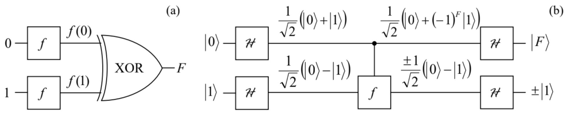
Classically, this is clearly impossible, and the simplest way to perform the function’s classification involves two similar black boxes \(f\) - see Fig. 4a. \(5^{0}\) It also uses the so-called exclusive-OR (XOR for short) gate whose output is described by the following function \(F\) of its two Boolean arguments \(j_{1}\) and \(j_{2}:^{51}\) \[F\left(j_{1}, j_{2}\right)=j_{1} \oplus j_{2} \equiv \begin{cases}0, & \text { if } j_{1}=j_{2}, \\ 1, & \text { if } j_{1} \neq j_{2} .\end{cases}\] In the particular circuit shown in Fig. 4a, the gate produces the following output: \[F=f(0) \oplus f(1) \text {, }\] which is equal to 1 if \(f(0) \neq f(1)\), i.e. if the function \(f\) is balanced, and to 0 in the opposite case - see column \(F\) in the table of Eq. (141).

Fig. 8.4. The simplest (a) classical and (b) quantum ways to classify a single-bit Boolean function \(f\).

On the other hand, as will be shown below, any of four functions \(f\) may be implemented quantum-mechanically, for example (Fig. 5a) as a unitary transform of two input qubits, acting as follows on each basis component \(\left.\left|j_{1} j_{2}\right\rangle \equiv\left|j_{1}\right\rangle j_{2}\right\rangle\) of the general input state (134): \[\hat{f}\left|j_{1}\right\rangle\left|j_{2}\right\rangle=\left|j_{1}\right\rangle\left|j_{2} \oplus f\left(j_{1}\right)\right\rangle,\] where \(f\) is the corresponding classical Boolean function - see the table in Eq. (141).

Fig. 8.5. Two-qubit quantum gates: (a) a two-qubit function \(f\) and (b) its particular case \(C\) (CNOT), and their actions on a basis state.

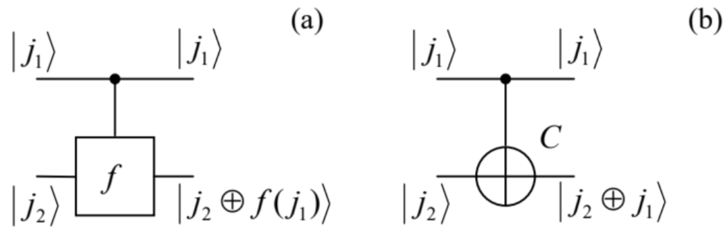
In the particular case when \(f\) in Eq. (144) is just the YES function: \(f(j)=f_{2}(j)=j\), this "circuit" is reduced to the so-called CNOT gate, a key ingredient of many other quantum computation schemes, performing the following two-qubit transform: \[\hat{C}\left|j_{1} j_{2}\right\rangle=\left|j_{1}\right\rangle\left|j_{2} \oplus j_{1}\right\rangle\] Let us use Eq. (142) to spell out this function for all four possible input qubit combinations: \[\hat{C}|00\rangle=|00\rangle, \quad \hat{C}|01\rangle=|01\rangle, \quad \hat{C}|10\rangle=|11\rangle, \quad \hat{C}|11\rangle=|10\rangle .\] In plain English, this means that acting on a basis state \(j_{1} j_{2}\), the CNOT gate leaves the state of the first, source qubit (shown by the upper horizontal line in Fig. 5) intact, but flips the state of the second, target qubit if the first one is in the basis state 1 . In even simpler words, the state \(j_{1}\) of the source qubit controls the NOT function acting on the target qubit; hence the gate’s name CNOT - the semi-acronym of "Controlled NOT".

For the quantum function (144), with an arbitrary and unknown \(f\), the Deutsch problem may be solved within the general scheme shown in Fig. 3, with the particular structure of the unitary-transform box \(U\) spelled out in Fig. \(4 \mathrm{~b}\), which involves just one implementation of the function \(f\). Here the singlequbit quantum gate #f performs the Hadamard (or "Walsh-Hadamard" or "Walsh") transform, \({ }^{52}\) whose operator is defined by the following actions on the qubit’s basis states: \[\hat{H}|0\rangle=\frac{1}{\sqrt{2}}(|0\rangle+|1\rangle), \quad \hat{H}|1\rangle=\frac{1}{\sqrt{2}}(|0\rangle-|1\rangle),\]

• see also the two leftmost state label columns in Fig. \(4 \mathrm{~b} .{ }^{53}\) Since this operator has to be linear (to be quantum-mechanically realistic), it needs to perform the action (146) on the basis states even when they are parts of a linear superposition - as they are, for example, for the two right Hadamard gates in Fig. 4b. For example, as immediately follows from Eqs. (146) and the operator’s linearity,

\[\hat{H}(\hat{H}|0\rangle)=\hat{H}\left(\frac{1}{\sqrt{2}}(|0\rangle+|1\rangle)\right)=\frac{1}{\sqrt{2}} \hat{H}(|0\rangle+\hat{H}|1\rangle)=\frac{1}{\sqrt{2}}\left(\frac{1}{\sqrt{2}}(|0\rangle+|1\rangle)+\frac{1}{\sqrt{2}}(|0\rangle-|1\rangle)\right)=|0\rangle .\] Absolutely similarly, we may get \(^{54}\) \[\hat{H}(\hat{H}|1\rangle)=|1\rangle \text {. }\] Now let us carry out a sequential analysis of the "circuit" shown in Fig. 4b. Since the input states of the gate \(f\) in this particular circuit are described by Eqs. (146), its output state’s ket is \[\hat{f}(\hat{\hat{f}}|0\rangle \hat{\mathcal{H}}|1\rangle)=\hat{f}\left(\frac{1}{\sqrt{2}}(|0\rangle+|1\rangle) \frac{1}{\sqrt{2}}(|0\rangle-|1\rangle)\right)=\frac{1}{2}(\hat{f}|00\rangle-\hat{f}|01\rangle+\hat{f}|10\rangle-\hat{f}|11\rangle) \text {. }\] Now we may apply Eq. (144) to each component in the parentheses: \[\begin{aligned} \hat{f}|00\rangle-\hat{f}|01\rangle+\hat{f}|10\rangle-\hat{f}|11\rangle & \equiv \hat{f}|0\rangle|0\rangle-\hat{f}|0\rangle|1\rangle+\hat{f}|1\rangle|0\rangle-\hat{f}|1\rangle|1\rangle \\ &=|0\rangle|0 \oplus f(0)\rangle-|0\rangle|1 \oplus f(0)\rangle+|1\rangle|0 \oplus f(1)\rangle-|1\rangle|1 \oplus f(1)\rangle \\ & \equiv|0\rangle(|0 \oplus f(0)\rangle-|1 \oplus f(0)\rangle)+|1\rangle(|0 \oplus f(1)\rangle-|1 \oplus f(1)\rangle) . \end{aligned}\] Note that the contents of the first parentheses of the last expression, characterizing the state of the target qubit, is equal to \((|0\rangle-|1\rangle) \equiv(-1)^{0}(|0\rangle-|1\rangle)\) if \(f(0)=0\) (and hence \(0 \oplus f(0)=0\) and \(\left.1 \oplus f(0)=1\right)\), and to \((|1\rangle\) \(-|0\rangle) \equiv(-1)^{1}(|0\rangle-|1\rangle)\) in the opposite case \(f(0)=1\), so that both cases may be described in one shot by rewriting the parentheses as \((-1)^{(0)}(|0\rangle-|1\rangle)\). The second parentheses is absolutely similarly controlled by the value of \(f(1)\), so that the outputs of the gate \(f\) are unentangled: \[\left.\hat{f}(\hat{\mathcal{H}}|0\rangle \hat{\mathcal{H}}|1\rangle)=\frac{1}{2}\left((-1)^{f(0)}|0\rangle+(-1)^{f(1)}|1\rangle\right)(0\rangle-|1\rangle\right)=\pm \frac{1}{\sqrt{2}}\left(|0\rangle+(-1)^{F}|1\rangle\right) \frac{1}{\sqrt{2}}(|0\rangle-|1\rangle),\] where the last step has used the fact that the classical Boolean function \(F\), defined by Eq. (142), is equal to \(\pm[f(1)-f(0)]-\) please compare the last two columns in Eq. (141). The front sign \(\pm\) in Eq. (150) may be prescribed to any of the component ket-vectors - for example to that of the target qubit, as shown by the third column of state labels in Fig. \(4 \mathrm{~b}\).

This intermediate result is already rather remarkable. Indeed, it shows that, despite the superficial impression one could get from Fig. 5, the gates \(f\) and \(C\), being "controlled" by the source qubit, may change that qubit’s state as well! This fact (partly reflected by the vertical direction of the control lines in Figs. 4 and 5, symbolizing the same stage of the system’s time evolution) shows how careful one should be interpreting quantum-computational "circuits", thriving on qubits’ entanglement, because the "signals" on different sections of a "wire" may differ-see Fig. \(4 b\) again.

At the last stage of the circuit shown in Fig. \(4 \mathrm{~b}\), the qubit components of the state \((150)\) are fed into one more pair of Hadamard gates, whose outputs therefore are \[\hat{H} \frac{1}{\sqrt{2}}\left(|0\rangle+(-1)^{F}|1\rangle\right)=\frac{1}{\sqrt{2}}\left(\hat{H}|0\rangle+(-1)^{F} \hat{H}|1\rangle\right), \quad \text { and } \hat{H}\left(\pm \frac{1}{\sqrt{2}}(|0\rangle-|1\rangle)\right)=\pm \frac{1}{\sqrt{2}}(\hat{H}|1\rangle-\hat{H}|0\rangle) .\] Now using Eqs. (146) again, we see that the output state ket-vectors of the source and target qubits are, respectively, \[\frac{1+(-1)^{F}}{2}|0\rangle+\frac{1-(-1)^{F}}{2}|1\rangle, \quad \text { and } \pm|1\rangle .\] Since, according to Eq. (142), the Boolean function \(F\) may take only values 0 or 1 , the final state of the source qubit is always one of its basis states \(j\), namely the one with \(j=F\). Its measurement tells us whether the function \(f\), participating in Eq. (144), is constant or balanced - see Eq. (141) again. \({ }^{55}\)

Thus, the quantum circuit shown in Fig. \(4 b\) indeed solves the Deutsch problem in one shot. Reviewing our analysis, we may see that this is possible because the unitary transform performed by the quantum gate \(f\) is applied to the entangled states (146) rather than to the basis states. Due to this trick, the quantum state components depending on \(f(0)\) and \(f(1)\) are processed simultaneously, in parallel. This quantum parallelism may be extended to circuits with many \((N>>1)\) qubits and, for some tasks, provide a dramatic performance increase - for example, reducing the necessary circuit component number from \(O\left(2^{N}\right)\) to \(O\left(N^{p}\right)\), where \(p\) is a finite (and not very big) number.

However, this efficiency comes at a high price. Indeed, let us discuss the possible physical implementation of quantum gates, starting from the single-qubit case, on an example of the Hadamard gate (146). With the linearity requirement, its action on the arbitrary state (133) should be \[\hat{\mathcal{H}}|\alpha\rangle=a_{0} \hat{\mathcal{H}}|0\rangle+a_{1} \hat{\mathcal{H}}|1\rangle=a_{0} \frac{1}{\sqrt{2}}(|0\rangle+|1\rangle)+a_{1} \frac{1}{\sqrt{2}}(|0\rangle-|1\rangle)=\frac{1}{\sqrt{2}}\left(a_{0}+a_{1}\right)|0\rangle+\frac{1}{\sqrt{2}}\left(a_{0}-a_{1}\right)|1\rangle,\] meaning that the state probability amplitudes in the end \((t=\tau)\) and in the beginning \((t=0)\) of the qubit evolution in time have to be related as \[a_{0}(\tau)=\frac{a_{0}(0)+a_{1}(0)}{\sqrt{2}}, \quad a_{1}(\tau)=\frac{a_{0}(0)-a_{1}(0)}{\sqrt{2}} .\] This task may be again performed using the Rabi oscillations, which were discussed in Sec. 6.5, i.e. by applying to the qubit (a two-level system), for a limited time period \(T\), a weak sinusoidal external signal of frequency \(\omega\) equal to the intrinsic quantum oscillation frequency \(\omega_{n n}\) ’ defined by Eq. (6.85). The analysis of the Rabi oscillations was carried out in Sec. 6.5, even for non-vanishing (though small) detuning \(\Delta=\omega-\omega_{n n}\), but only for the particular initial conditions when at \(t=0\) the system was fully in one on the basis states (there labeled as \(n\) ’), i.e. the counterpart state (there labeled \(n\) ) was empty. For our current purposes we need to find the amplitudes \(a_{0,1}(t)\) for arbitrary initial conditions \(a_{0,1}(0)\), subject only to the time-independent normalization condition \(\left|a_{0}\right|^{2}+\left|a_{1}\right|^{2}=1\). For the case of exact tuning, \(\Delta=\) 0 , the solution of the system (6.94) is elementary, \({ }^{56}\) and gives the following solution: \({ }^{57}\) \[\begin{aligned} &a_{0}(t)=a_{0}(0) \cos \Omega t-i a_{1}(0) e^{i \varphi} \sin \Omega t, \\ &a_{1}(t)=a_{1}(0) \cos \Omega t-i a_{0}(0) e^{-i \varphi} \sin \Omega t, \end{aligned}\] where \(\Omega\) is the Rabi oscillation frequency (6.99), in the exact-tuning case proportional to the amplitude \(|A|\) of the external ac drive \(A=|A| \exp \{i \varphi\}-\) see Eq. (6.86). Comparing these expressions with Eqs. (154), we see that for \(t=\tau=\pi / 4 \Omega\) and \(\varphi=\pi / 2\) they "almost" coincide, besides the opposite sign of \(a_{1}(\tau)\). Conceptually the simplest way to correct this deficiency is to follow the \(a c\) " \(\pi / 4\)-pulse", just discussed, by a short \(d c\) " \(\pi\)-pulse" of the duration \(\mathcal{T}=\pi / \delta\), which temporarily creates a small additional energy difference \(\delta\) between the basis states 0 and 1. According to the basic Eq. (1.62), such difference creates an additional phase difference \(\tau \delta / \hbar\) between the states, equal to \(\pi\) for the " \(\pi\)-pulse".

Another way (that may be also useful for two-qubit operations) is to use another, auxiliary energy level \(E_{2}\) whose distances from the basic levels \(E_{1}\) and \(E_{0}\) are significantly different from the difference \(\left(E_{1}-E_{0}\right)-\) see Fig. 6a. In this case, the weak external ac field tuned to any of the three potential quantum transition frequencies \(\omega_{n n^{\prime}} \equiv\left(E_{n^{-}} E_{n^{\prime}}\right) / \hbar\) initiates such transitions between the corresponding states only, with a negligible perturbation of the third state. (Such transitions may be again described by Eqs. (155), with the appropriate index changes.) For the Hadamard transform implementation, it is sufficient to apply (after the already discussed \(\pi / 4\)-pulse of frequency \(\omega_{10}\), and with the initially empty level \(E_{2}\) ), an additional \(\pi\)-pulse of frequency \(\omega_{20}\), with any phase \(\varphi\). Indeed, according to the first of Eqs. (155), with the due replacement \(a_{1}(0) \rightarrow a_{2}(0)=0\), such pulse flips the sign of the amplitude \(a_{0}(t)\), while the amplitude \(a_{1}(t)\), not involved in this additional transition, remains unchanged.

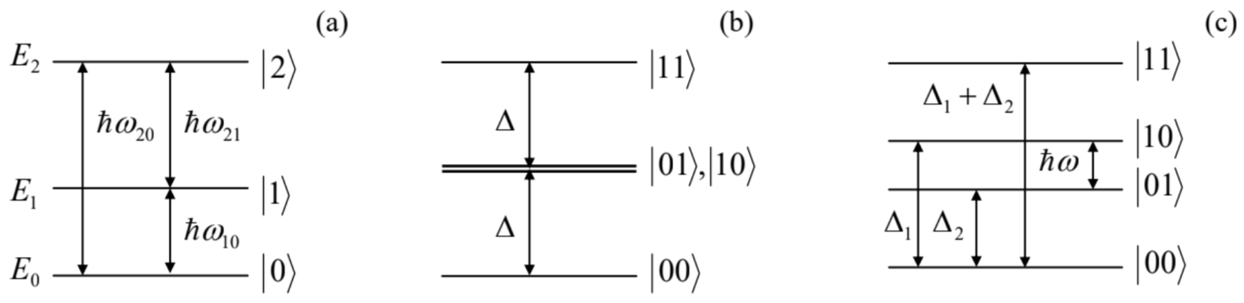Fig. 8.6. Energy-level schemes used for unitary transformations of (a) single qubits and (b, c) two-qubit systems.

Now let me describe the conceptually simplest (though, for some qubit types, not the most practically convenient) scheme for the implementation of two-qubit gates, on an example of the CNOT gate whose operation is described by Eq. (145). For that, evidently, the involved qubits have to interact for some time \(T\). As was repeatedly discussed in the two last chapters, in most cases such interaction of two subsystems is factorable - see Eq. (6.145). For qubits, i.e. two-level systems, each of the component operators may be represented by a \(2 \times 2\) matrix in the basis of states 0 and 1 . According to Eq. (4.106), such matrix may be always expressed as a linear combination \((b \mathrm{I}+\mathbf{c} \cdot \boldsymbol{\sigma})\), where \(b\) and three Cartesian components of the vector \(\mathbf{c}\) are \(c\)-numbers. Let us consider the simplest form of such factorable interaction Hamiltonian: \[\hat{H}_{\mathrm{int}}(t)=\left\{\begin{array}{cc} \kappa \hat{\sigma}_{z}^{(1)} \hat{\sigma}_{z}^{(2)}, & \text { for } 0<t<\tau \\ 0, & \text { otherwise, } \end{array}\right.\] where the upper index is the qubit number and \(\kappa\) is a \(c\)-number constant. \({ }^{58}\) According to Eq. (4.175), by the end of the interaction period, this Hamiltonian produces the following unitary transform: \[\hat{U}_{\mathrm{int}}=\exp \left\{-\frac{i}{\hbar} \hat{H}_{\mathrm{int}} \tau\right\} \equiv \exp \left\{-\frac{i}{\hbar} \kappa \hat{\sigma}_{z}^{(1)} \hat{\sigma}_{z}^{(2)} \tau\right\} .\] Since in the basis of unperturbed two-bit basis states \(\left|j_{1} j_{2}\right\rangle\), the product operator \(\hat{\sigma}_{z}^{(1)} \hat{\sigma}_{z}^{(2)}\) is diagonal, so is the unitary operator (157), with the following action on these states:

\[\hat{U}_{\text {int }}\left|j_{1} j_{2}\right\rangle=\exp \left\{i \theta \sigma_{z}^{(1)} \sigma_{z}^{(2)}\right\}\left|j_{1} j_{2}\right\rangle,\] where \(\theta \equiv-\kappa \pi \hbar\), and \(\sigma_{z}\) are the eigenvalues of the Pauli matrix \(\sigma_{\mathrm{z}}\) for the basis states of the corresponding qubit: \(\sigma_{z}=+1\) for \(|j\rangle=|0\rangle\), and \(\sigma_{z}=-1\) for \(|j\rangle=|1\rangle\). Let me, for clarity, spell out Eq. (158) for the particular case \(\theta=-\pi / 4\) (corresponding to the qubit coupling time \(\tau=\pi \hbar / 4 \kappa\) ): \[\hat{U}_{\text {int }}|00\rangle=e^{-i \pi / 4}|00\rangle, \quad \hat{U}_{\text {int }}|01\rangle=e^{i \pi / 4}|01\rangle, \quad \hat{U}_{\text {int }}|10\rangle=e^{i \pi / 4}|10\rangle, \quad \hat{U}_{\text {int }}|11\rangle=e^{-i \pi / 4}|11\rangle .\] In order to compensate the undesirable parts of this joint phase shift of the basis states, let us now apply similar individual "rotations" of each qubit by angle \(\theta\) ’ \(=+\pi / 4\), using the following product of two independent operators, plus (just for the result’s clarity) a common, and hence inconsequential, phase shift \(\theta^{\prime \prime}=-\pi / 4: 59\) \[\hat{U}_{\text {com }}=\exp \left\{i \theta^{\prime}\left(\hat{\sigma}_{z}^{(1)}+\hat{\sigma}_{z}^{(2)}\right)+i \theta^{\prime \prime}\right\} \equiv \exp \left\{i \frac{\pi}{4} \hat{\sigma}_{z}^{(1)}\right\} \exp \left\{i \frac{\pi}{4} \hat{\sigma}_{z}^{(2)}\right\} e^{-i \pi / 4} .\] Since this operator is also diagonal in the \(\left|j_{j} j_{2}\right\rangle\) basis, it is easy to calculate the change of the basis states by the total unitary operator \(\hat{U}_{\text {tot }} \equiv \hat{U}_{\text {com }} \hat{U}_{\text {int }}\) : \[\hat{U}_{\mathrm{tot}}|00\rangle=|00\rangle, \quad \hat{U}_{\mathrm{tot}}|01\rangle=|01\rangle, \quad \hat{U}_{\mathrm{tot}}|10\rangle=|10\rangle, \quad \hat{U}_{\mathrm{tot}}|11\rangle=-|11\rangle .\] This result already shows the main "miracle action" of two-qubit gates, such as the one shown in Fig. \(4 \mathrm{~b}\) : the source qubit is left intact (only if it is in one of the basis states!), while the state of the target qubit is altered. True, this change (of the sign) is still different from the CNOT operator’s action (145), but may be readily used for its implementation by sandwiching of the transform \(U_{\text {tot }}\) between two Hadamard transforms of the target qubit alone: \[\hat{C}=\frac{1}{2} \hat{H}^{(2)} \hat{U}_{\mathrm{tot}} \hat{H}^{(2)}\] So, we have spent quite a bit of time on the discussion of the CNOT gate, \({ }^{60}\) and now I can reward the reader for their effort with a bit of good news: it has been proved that an arbitrary unitary transform that satisfies Eq. (140), i.e. may be used within the general scheme outlined in Fig. 3, may be decomposed into a set of CNOT gates, possibly augmented with simpler single-qubit gates - for example, the Hadamard gate plus the \(\pi / 2\) rotation discussed above. \({ }^{61}\) Unfortunately, I have no time for a detailed discussion of more complex circuits. \({ }^{62}\) The most famous of them is the scheme for integer number factoring, suggested in 1994 by Peter Winston Shor. \({ }^{63}\) Due to its potential practical importance for breaking broadly used communication encryption schemes such as the RSA code, \({ }^{64}\) this opportunity has incited much enthusiasm and triggered experimental efforts to implement quantum gates and circuits using a broad variety of two-level quantum systems. By now, the following experimental options have given the most significant results: \({ }^{65}\)

(i) Trapped ions. The first experimental demonstrations of quantum state manipulation (including the already mentioned first CNOT gate) have been carried out using deeply cooled atoms in optical traps, similar to those used in frequency and time standards. Their total spins are natural qubits, whose states may be manipulated using the Rabi transfers excited by suitably tuned lasers. The spin interactions with the environment may be very weak, resulting in large dephasing times \(T_{2}-\) up to a few seconds. Since the distances between ions in the traps are relatively large (of the order of a micron), their direct spin-spin interaction is even weaker, but the ions may be made effectively interacting either via their mechanical oscillations about the potential minima of the trapping field, or via photons in external electromagnetic resonators ("cavities"). \({ }^{66}\) Perhaps the main challenge of using this approach for quantum computation is poor "scalability", i.e. the enormous experimental difficulty of creating and managing large ordered systems of individually addressable qubits. So far, only a-few-qubit systems have been demonstrated. \({ }^{67}\)

(ii) Nuclear spins are also typically very weakly connected to their environment, with dephasing times \(T_{2}\) exceeding 10 seconds in some cases. Their eigenenergies \(E_{0}\) and \(E_{1}\) may be split by external dc magnetic fields (typically, of the order of \(10 \mathrm{~T}\) ), while the interstate Rabi transfers may be readily achieved by using the nuclear magnetic resonance, i.e. the application of external ac fields with frequencies \(\omega=\left(E_{1}-E_{0}\right) / \hbar\) - typically, of a few hundred \(\mathrm{MHz}\). The challenges of this option include the weakness of spin-spin interactions (typically mediated through molecular electrons), resulting in a very slow spin evolution, whose time scale \(\hbar / \kappa\) may become comparable with \(T_{2}\), and also very small level separations \(E_{1}-E_{0}\), corresponding to a few K, i.e. much smaller than the room temperature, creating a challenge of qubit state preparation. \({ }^{68}\) Despite these challenges, the nuclear spin option was used for the first implementation of the Shor algorithm for factoring of a small number \((15=5 \times 3)\) as early as \(2001.69\) However, the extension of this success to larger systems, beyond the set of spins inside one molecule, is extremely challenging.

(iii) Josephson-junction devices. Much better scalability may be achieved with solid-state devices, especially using superconductor integrated circuits including weak contacts - Josephson junctions (see their brief discussion in Sec. 1.6). The qubits of this type are based on the fact that the energy \(U\) of such a junction is a highly nonlinear function of the Josephson phase difference \(\varphi\) - see Sec. 1.6. Indeed, combining Eqs. (1.73) and (1.74), we can readily calculate \(U(\varphi)\) as the work \(\mathscr{W}\) of an external circuit increasing the phase from, say, zero to some value \(\varphi\) : \[U(\varphi)-U(0)=\int_{\varphi^{\prime}=0}^{\varphi^{\prime}=\varphi} d \mathscr{W}=\int_{\varphi^{\prime}=0}^{\varphi^{\prime}=\varphi} I V d t=\frac{2 e I_{\mathrm{c}}}{\hbar} \int_{\varphi^{\prime}=0}^{\varphi^{\prime}=\varphi} \sin \varphi^{\prime} \frac{d \varphi^{\prime}}{d t} d t=\frac{2 e I_{\mathrm{c}}}{\hbar}(1-\cos \varphi) .\] There are several options of using this nonlinearity for creating qubits; \({ }^{70}\) currently the leading option, called the phase qubit, is using two lowest eigenstates localized in one of the potential wells of the periodic potential (163). A major problem of such qubits is that at the very bottom of this well the potential \(U(\varphi)\) is almost quadratic, so that the energy levels are nearly equidistant - cf. Eqs. (2.262), (6.16), and (6.23). This is even more true for the so-called "transmons" (and "Xmons", and "Gatemons", and several other very similar devices \({ }^{71}\) ) - the currently used phase qubits versions, where a Josephson junction is made a part of an external electromagnetic oscillator, making its relative total nonlineartity (anharmonism) even smaller. As a result, the external rf drive of frequency \(\omega=\left(E_{1}-E_{0}\right) / \hbar\), used to arrange the state transforms described by Eq. (155), may induce simultaneous undesirable transitions to (and between) higher energy levels. This effect may be mitigated by a reduction of the ac drive amplitude, but at a price of the proportional increase of the operation time and hence of dephasing - see below. (I am leaving a quantitative estimate of such an increase for the reader’s exercise.)

Since the coupling of Josephson-junction qubits may be most readily controlled (and, very importantly, kept stable if so desired), they have been used to demonstrate the largest prototype quantum computing systems to date, despite quite modest dephasing times \(T_{2}-\) for purely integrated circuits, in the tens of microseconds at best, even at operating temperatures in tens of \(\mathrm{mK}\). By the time of this writing (mid-2019), several groups have announced chips with a few dozen of such qubits, but to the best of my knowledge, only their smaller subsets could be used for high-fidelity quantum operations. \({ }^{72}\)

(iv) Optical systems, attractive because of their inherently enormous bandwidth, pose a special challenge for quantum computation: due to the virtual linearity of most electromagnetic media at reasonable light power, the implementation of qubits (i.e. two-level systems), and interaction Hamiltonians such as the one given by Eq. (156), is problematic. In 2001, a very smart way around this hurdle was invented. \({ }^{73}\) In this KLM scheme (also called the "linear optical quantum computing"), nonlinear elements are not needed at all, and quantum gates may be composed just of linear devices (such as optical waveguides, mirrors, and beam splitters), plus single-photon sources and detectors. However, estimates show that this approach requires a much larger number of physical components than those using nonlinear quantum systems such as usual qubits, \({ }^{74}\) so that right now it is not very popular.

So, despite more than two decades of large-scale efforts, the progress of quantum computing development has been rather modest. The main culprit here is the unintentional coupling of qubits to their environment, leading most importantly to their state dephasing, and eventually to errors. Let me discuss this major issue in detail.

Of course, some error probability exists in classical digital logic gates and memory cells as well. \({ }^{75}\) However, in this case, there is no conceptual problem with the device state measurement, so that the error may be detected and corrected in many ways. Conceptually, \({ }^{76}\) the simplest of them is the socalled majority voting logic - using several similar logic circuits working in parallel and fed with identical input data. Evidently, two such devices can detect a single error in one of them, while three devices in parallel may correct such error, by taking two coinciding output signals for the genuine one.

For quantum computation, the general idea of using several devices (say, qubits) for coding the same information remains valid; however, there are two major complications. First, as we know from Chapter 7 , the environment’s dephasing effect may be described as a slow random drift of the probability amplitudes \(a_{j}\), leading to the deviation of the output state \(\alpha_{\text {fin }}\) from the required form (140), and hence to a non-vanishing probability of wrong qubit state readout - see Fig. 3. Hence the quantum error correction has to protect the result not against possible random state flips \(0 \leftrightarrow 1\), as in classical digital computers, but against these "creeping" analog errors.

Second, the qubit state is impossible to copy exactly (clone) without disturbing it, as follows from the following simple calculation. \({ }^{77}\) Cloning some state \(\alpha\) of one qubit to another qubit that is initially in an independent state (say, the basis state 0 ), without any change of \(\alpha\), means the following transformation of the two-qubit ket: \(|\alpha 0\rangle \rightarrow|\alpha \alpha\rangle\). If we want such transform to be performed by a real quantum system, whose evolution is described by a unitary operator \(\hat{u}\), and to be correct for an arbitrary state \(\alpha\), it has to work not only for both basis states of the qubit: \[\hat{u}|00\rangle=|00\rangle, \quad \hat{u}|10\rangle=|11\rangle,\] but also for their arbitrary linear combination (133). Since the operator \(\hat{u}\) has to be linear, we may use that relation, and then Eq. (164) to write \[\hat{u}|\alpha 0\rangle \equiv \hat{u}\left(a_{0}|0\rangle+a_{1}|1\rangle\right)|0\rangle \equiv a_{0} \hat{u}|00\rangle+a_{1} \hat{u}|10\rangle=a_{0}|00\rangle+a_{1}|11\rangle .\] On the other hand, the desired result of the state cloning is \[|\alpha \alpha\rangle=\left(a_{0}|0\rangle+a_{1}|1\rangle\right)\left(a_{0}|0\rangle+a_{1}|1\rangle\right) \equiv a_{0}^{2}|00\rangle+a_{0} a_{1}(|10\rangle+|01\rangle)+a_{1}^{2}|11\rangle,\] i.e. is evidently different, so that, for an arbitrary state \(\alpha\), and an arbitrary unitary operator \(\hat{u}\), \[\hat{u}|\alpha 0\rangle \neq|\alpha \alpha\rangle,\] meaning that the qubit state cloning is indeed impossible. \({ }^{78}\) This problem may be, however, indirectly circumvented - for example, in the way shown in Fig. \(7 \mathrm{a}\).

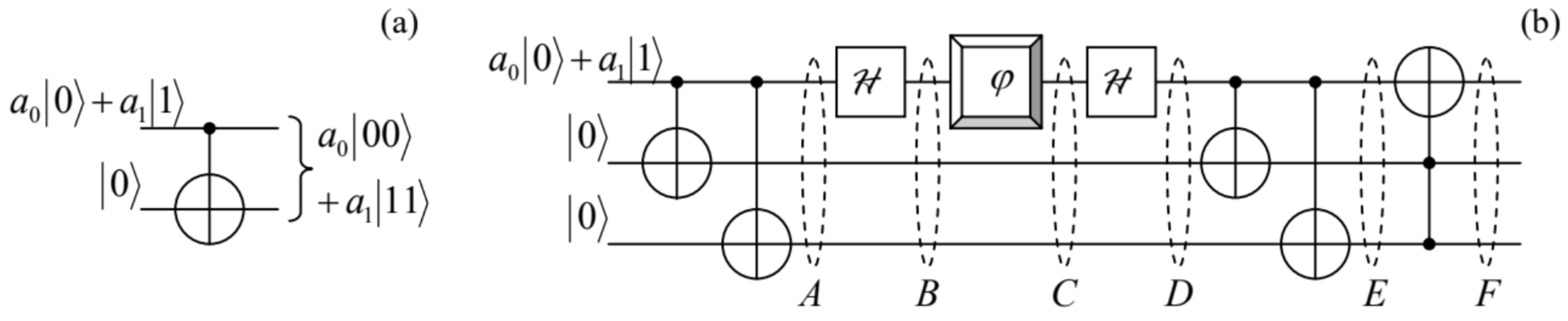Fig. 8.7. (a) Quasi-cloning, and (b) detection and correction of dephasing errors in a single qubit.

Here the CNOT gate, whose action is described by Eq. (145), entangles an arbitrary input state (133) of the source qubit with a basis initial state of an ancillary target qubit - frequently called the ancilla. Using Eq. (145), we can readily calculate the output two-qubit state’s vector: \[|\alpha\rangle_{N=2}=\hat{C}\left(a_{0}|0\rangle+a_{1}|1\rangle\right)|0\rangle \equiv a_{0} \hat{C}|00\rangle+a_{1} \hat{C}|10\rangle=a_{0}|00\rangle+a_{1}|11\rangle\] We see that this circuit does perform the operation (165), i.e. gives the initial source qubit’s probability amplitudes \(a_{0}\) and \(a_{1}\) equally to two qubits, i.e. duplicates the input information. However, in contrast with the "genuine" cloning, it changes the state of the source qubit as well, making it entangled with the target (ancilla) qubit. Such "quasi-cloning" is the key element of most suggested quantum error correction techniques.

Consider, for example, the three-qubit "circuit" shown in Fig. \(7 \mathrm{~b}\), which uses two ancilla qubits - see the two lower "wires". At its first two stages, the double application of the quasi-cloning produces an intermediate state \(A\) with the following ket-vector: \[|A\rangle=a_{0}|000\rangle+a_{1}|111\rangle,\] which is an evident generalization of Eq. (168). \({ }^{79} \mathrm{Next}\), subjecting the source qubit to the Hadamard transform (146), we get the three-qubit state \(B\) represented by the state vector

\[|B\rangle=a_{0} \frac{1}{\sqrt{2}}(|0\rangle+|1\rangle)|00\rangle+a_{1} \frac{1}{\sqrt{2}}(|0\rangle-|1\rangle)|11\rangle .\] Now let us assume that at this stage, the source qubit comes into contact with a dephasing environment - in Fig. \(7 \mathrm{~b}\), symbolized by the single-qubit "gate" \(\varphi\). As we know from Chapter 7 (see Eq. (7.22) and its discussion, and also Sec. 7.3), its effect may be described by a random shift of the relative phase of two states: \({ }^{80}\) \[|0\rangle \rightarrow e^{i \varphi}|0\rangle, \quad|1\rangle \rightarrow e^{-i \varphi}|1\rangle\] As a result, for the intermediate state \(C\) (see Fig. \(7 \mathrm{~b}\) ) we may write \[|C\rangle=a_{0} \frac{1}{\sqrt{2}}\left(e^{i \varphi}|0\rangle+e^{-i \varphi}|1\rangle\right)|00\rangle+a_{1} \frac{1}{\sqrt{2}}\left(e^{i \varphi}|0\rangle-e^{-i \varphi}|1\rangle\right)|11\rangle .\] At this stage, in this simple theoretical model, the coupling with the environment is completely stopped (ahh, if this could be possible! we might have quantum computers by now :-), and the source qubit is fed into one more Hadamard gate. Using Eqs. (146) again, for the state \(D\) after this gate we get \[|D\rangle=a_{0}(\cos \varphi|0\rangle+i \sin \varphi|1\rangle)|00\rangle+a_{1}(i \sin \varphi|0\rangle+\cos \varphi|1\rangle)|11\rangle .\] Now the qubits are passed through the second, similar pair of CNOT gates - see Fig. 7b. Using Eq. (145), for the resulting state \(E\) we readily get the following expression: \[|E\rangle=a_{0} \cos \varphi|000\rangle+a_{0} i \sin \varphi|111\rangle+a_{1} i \sin \varphi|011\rangle+a_{1} \cos \varphi|100\rangle,\] whose right-hand side may by evidently grouped as \[|E\rangle=\left(a_{0}|0\rangle+a_{1}|1\rangle\right) \cos \varphi|00\rangle+\left(a_{1}|0\rangle+a_{0}|1\rangle\right) i \sin \varphi|11\rangle .\] This is already a rather remarkable result. It shows that if we measured the ancilla qubits at stage \(E\), and both results corresponded to states 0 , we might be \(100 \%\) sure that the source qubit (which is not affected by these measurements!) is in its initial state even after the interaction with the environment. The only result of an increase of this unintentional interaction (as quantified by the r.m.s. magnitude of the random phase shift \(\varphi\) ) is the growth of the probability, \[W=\sin ^{2} \varphi\] of getting the opposite result, which signals a dephasing-induced error in the source qubit. Such implicit measurement, without disturbing the source qubit, is called quantum error detection.

An even more impressive result may be achieved by the last component of the circuit, the socalled Toffoli (or "CCNOT") gate, denoted by the rightmost symbol in Fig. 7b. This three-qubit gate is conceptually similar to the CNOT gate discussed above, besides that it flips the basis state of its target qubit only if both source qubits are in state 1. (In the circuit shown in Fig. \(7 \mathrm{~b}\), the former role is played by our source qubit, while the latter role, by the two ancilla qubits.) According to its definition, the Toffoli gate does not affect the first parentheses in Eq. (174b), but flips the source qubit’s states in the second parentheses, so that for the output three-qubit state \(F\) we get \[|F\rangle=\left(a_{0}|0\rangle+a_{1}|1\rangle\right) \cos \varphi|00\rangle+\left(a_{0}|0\rangle+a_{1}|1\rangle\right) i \sin \varphi|11\rangle \text {. }\] Obviously, this result may be factored as \[|F\rangle=\left(a_{0}|0\rangle+a_{1}|1\rangle\right)(\cos \varphi|00\rangle+i \sin \varphi|11\rangle),\] showing that now the source qubit is again fully unentangled from the ancilla qubits. Moreover, Quantum calculating the norm squared of the second operand, we get \[\left(\operatorname { c o s } \varphi \left\langle00|-i \sin \varphi\langle 11|)(\cos \varphi|00\rangle+i \sin \varphi|11\rangle)=\cos ^{2} \varphi+\sin ^{2} \varphi=1\right.\right.\] so that the final state of the source qubit exactly coincides with its initial state. This is the famous miracle of quantum state correction, taking place "automatically" - without any qubit measurements, and for any random phase shift \(\varphi\).

The circuit shown in Fig. \(7 \mathrm{~b}\) may be further improved by adding Hadamard gate pairs, similar to that used for the source qubit, to the ancilla qubits as well. It is straightforward to show that if the dephasing is small in the sense that the \(W\) given by Eq. (175) is much less than 1, this modified circuit may provide a substantial error probability reduction (to \(\sim W^{2}\) ) even if the ancilla qubits are also subjected to a similar dephasing and the source qubits, at the same stage - i.e. between the two Hadamard gates. Such perfect automatic correction of any error (not only of an inner dephasing of a qubit and its relaxation/excitation, but also of the mutual dephasing between qubits) of any used qubit needs even more parallelism. The first circuit of that kind, based on nine parallel qubits, which is a natural generalization of the circuit discussed above, was invented in 1995 by the same P. Shor. Later, five-qubit circuits enabling similar error correction were suggested. (The further parallelism reduction has been proved impossible.)

However, all these results assume that the error correction circuits as such are perfect, i.e. completely isolated from the environment. In the real world, this cannot be done. Now the key question is what maximum level \(W_{\max }\) of the error probability in each gate (including those in the used error correction scheme) can be automatically corrected, and how many qubits with \(W<W_{\max }\) would be required to implement quantum computers producing important practical results - first of all, factoring of large numbers. \({ }^{81}\) To the best of my knowledge, estimates of these two related numbers have been made only for some very specific approaches, and they are rather pessimistic. For example, using the socalled surface codes, which employ many physical qubits for coding an informational one, and hence increase its fidelity, \(W_{\min }\) may be increased to a few times \(10^{-3}\), but then we would need \(\sim 10^{8}\) physical qubits for the Shor’s algorithm implementation. \({ }^{82}\) This is very far from what currently looks doable using the existing approaches.

Because of this hard situation, the current development of quantum computing is focused on finding at least some problems that could be within the reach of either the existing systems, or their immediate extensions, and simultaneously would present some practical interest - a typical example of a technology in the search for applications. Currently, to the best of my knowledge, all suggested problems of this kind address either specially crafted mathematical problems, \({ }^{83}\) or properties of some simple physical systems - such as the molecular hydrogen \({ }^{84}\) or the deuteron (the deuterium’s nucleus, i.e. the proton-neutron system). \({ }^{85}\) In the latter case, the interaction between the qubits of the computational system is organized so that the system’s Hamiltonian is similar to that of the quantum system of interest. (For this work, quantum simulation is a more adequate name than "quantum computation". \({ }^{86}\) )

Such simulations are pursued by some teams using schemes different from that shown in Fig. 3 . Of those, the most developed is the so-called adiabatic quantum computation, \({ }^{87}\) which drops the hardest requirement of negligible interaction with the environment. In this approach, the qubit system is first prepared in a certain initial state, and then is let evolve on its own, with no effort to couple-uncouple qubits by external control signals during the evolution. \({ }^{88}\) Due to the interaction with the environment, in particular the dephasing and the energy dissipation it imposes, the system eventually relaxes to a final incoherent state, which is then measured. (This reminds the scheme shown in Fig. 3, with the important difference that the transform \(U\) should not necessarily be unitary.) From numerous runs of such an experiment, the outcome statistics may be revealed. Thus, at this approach the interaction with the environment is allowed to play a certain role in the system evolution, though every effort is made to reduce it, thus slowing down the relaxation process - hence the word "adiabatic" in the name of this approach. This slowness allows the system to exhibit some quantum properties, in particular quantum tunneling 89 through the energy barriers separating close energy minima in the multi-dimensional space of states. This tunneling creates a substantial difference in the finite state statistics from that in purely classical systems, where such barriers may be overcome only by thermally-activated jumps over them. \({ }^{90}\)

Due to technical difficulties of the organization and precise control of long-range interaction in multi-qubit systems, the adiabatic quantum computing demonstrations so far have been limited to a few simple arrays described by the so-called extended quantum Ising ("spin-glass") model \[\hat{H}=-J \sum_{\{j, j\}} \hat{\sigma}_{z}^{(j)} \hat{\sigma}_{z}^{\left(j^{\prime}\right)}-\sum_{j} h_{j} \hat{\sigma}_{z}^{(j)},\] where the curly brackets denote the summation over pairs of close (though not necessarily closest) neighbors. Though the Hamiltonian (178) is the traditional playground of phase transitions theory (see, e.g., SM Chapter 4), to the best of my knowledge there are not many practically important tasks that could be achieved by studying the statistics of its solutions. Moreover, even for this limited task, the speed of the largest experimental adiabatic quantum "computers", with several hundreds of Josephsonjunction qubits \({ }^{91}\) is still comparable with that of classical, off-the-shelf semiconductor processors (with the dollar cost lower by many orders of magnitude), and no dramatic change of this comparison is predicted for realistic larger systems.

To summarize the current (circa mid-2019) situation with the quantum computation development, it faces a very hard challenge of mitigating the effects of unintentional coupling with the environment. This problem is exacerbated by the lack of algorithms, beyond Shor’s factoring, that would give quantum computation a substantial advantage over the classical competition in solving realworld problems, and hence a much broader potential customer base that would provide the field with the necessary long-term motivation and resources. So far, even the leading experts in this field abstain from predictions on when quantum computation may become a self-supporting commercial technology. \({ }^{92}\)

There seem to be somewhat better prospects for another application of entangled qubit systems, namely to telecommunication cryptography. \({ }^{93}\) The goal here is more modest: to replace the currently dominating classical encryption, based on the public-key RSA code mentioned above, that may be broken by factoring very large numbers, with a quantum encryption system that would be fundamentally unbreakable. The basis of this opportunity is the measurement postulate and the no-cloning theorem: if a message is carried over by a qubit, it is impossible for an eavesdropper (in cryptography, traditionally called Eve) to either measure or copy it faithfully, without also disturbing its state. However, as we have seen from the discussion of Fig. 7a, state quasi-cloning using entangled qubits is possible, so that the issue is far from being simple, especially if we want to use a publicly distributed quantum key, in some sense similar to the classical public key used at the RSA encryption. Unfortunately, I would not have time/space to discuss various options for quantum encryption, but cannot help demonstrating how counter-intuitive they may be, on the famous example of the so-called quantum teleportation (Fig. 8). \({ }^{94}\)

Suppose that some party A (in cryptography, traditionally called Alice) wants to send to party B (Bob) the full information about the pure quantum state \(\alpha\) of a qubit, unknown to either party. Instead of sending her qubit directly to Bob, Alice asks him to send her one qubit \((\beta)\) of a pair of other qubits, prepared in a certain entangled state, for example in the singlet state described by Eq. (11); in our current notation

\[\left|\beta \beta^{\prime}\right\rangle=\frac{1}{\sqrt{2}}(|01\rangle-|10\rangle) .\]

The initial state of the whole three-qubit system may be represented in the form

\[\left|\alpha \beta \beta^{\prime}\right\rangle=\left(a_{0}|0\rangle+a_{1}|1\rangle\right)\left|\beta \beta^{\prime}\right\rangle=\frac{a_{0}}{\sqrt{2}}|001\rangle-\frac{a_{0}}{\sqrt{2}}|010\rangle+\frac{a_{1}}{\sqrt{2}}|010\rangle-\frac{a_{1}}{\sqrt{2}}|111\rangle\]

which may be equivalently rewritten as the following linear superposition,

\[\begin{aligned} \left|\alpha \beta \beta^{\prime}\right\rangle &=\frac{1}{2}|\alpha \beta\rangle_{\mathrm{s}}^{+}\left(-a_{1}|0\rangle+a_{0}|1\rangle\right)+\frac{1}{2}|\alpha \beta\rangle_{\mathrm{s}}^{-}\left(a_{1}|0\rangle+a_{0}|1\rangle\right) \\ &+\frac{1}{2}|\alpha \beta\rangle_{\mathrm{e}}^{+}\left(-a_{0}|0\rangle+a_{1}|1\rangle\right)+\frac{1}{2}|\alpha \beta\rangle_{\mathrm{e}}^{-}\left(-a_{0}|0\rangle-a_{1}|1\rangle\right) \end{aligned}\]

of the following four states of the qubit pair \(\alpha \beta\):

\[|\alpha \beta\rangle_{\mathrm{s}}^{\pm} \equiv \frac{1}{\sqrt{2}}(|00\rangle \pm|11\rangle), \quad|\alpha \beta\rangle_{\mathrm{e}}^{\pm} \equiv \frac{1}{\sqrt{2}}(|01\rangle \pm|10\rangle) .\]

transfer of the qubit \(\ \beta\), (c) the measurement of the pair \(\ \alpha \beta\), (d) the forward transfer of two classical bits with the measurement results, and (e) the final state, with the state of the qubit \(\ \beta^{\prime}\) mirroring the initial state of the qubit \(\ \alpha\).

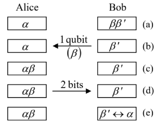
After having received qubit \(\beta\) from Bob, Alice measures which of these four states does the pair \(\alpha \beta\) have. This may be achieved, for example, by measurement of one observable represented by the operator \(\hat{\sigma}_{z}^{(\alpha)} \hat{\sigma}_{z}^{(\beta)}\) and another one corresponding to \(\hat{\sigma}_{x}^{(\alpha)} \hat{\sigma}_{x}^{(\beta)}-\) cf. Eq. (156). (Since all four states (181) are eigenstates of both these operators, these two measurements do not affect each other and may be performed in any order.) The measured eigenvalue of the former operator enables distinguishing the couples of states (181) with different values of the lower index, while the latter measurement distinguishes the states with different upper indices.

Then Alice reports the measurement result (which may be coded with just two classical bits) to Bob over a classical communication channel. Since the measurement places the pair \(\alpha \beta\) definitely into the corresponding state, the remaining Bob’s bit \(\beta\) ’ is now definitely in the unentangled single-qubit state that is represented by the corresponding parentheses in Eq. (180b). Note that each of these parentheses contains both coefficients \(a_{0,1}\), i.e. the whole information about the initial state that the qubit \(\alpha\) had initially. If Bob likes, he may now use appropriate single-qubit operations, similar to those discussed earlier in this section, to move his qubit \(\beta\) ’ into the state exactly similar to the initial state of qubit \(\alpha\). (This fact does not violate the no-cloning theorem (167), because the measurement has already changed the state of \(\alpha\).) This is, of course, a "teleportation" only in a very special sense of this term, but a good example of the importance of qubit entanglement’s preservation at their spatial transfer. For this course, this was also a good primer for the forthcoming discussion of the EPR paradox and Bell’s inequalities in Chapter \(10 .\) Returning for just a minute to quantum cryptography: since its most common quantum key distribution protocols \({ }^{95}\) require just a few simple quantum gates, whose experimental implementation is not a large technological challenge, the main focus of the current effort is on decreasing the singlephoton dephasing in long electromagnetic-wave transmission channels, \({ }^{9}\) with sufficiently high qubit transfer fidelity. The recent progress was rather impressive, with the demonstrated transfer of entangled qubits over landlines longer than \(100 \mathrm{~km},{ }^{97}\) and over at least one satellite-based line longer than 1,000 \(\mathrm{km} ; 98\) and also the whole quantum key distribution over a comparable distance, though for now at a very low rate yet. \({ }^{99}\) Let me hope that if not the author of this course, then its readers will see this technology used in practical secure telecommunication systems.

---

\({ }^{42}\) Despite the recent flood of new books on the field, one of its first surveys, by M. Nielsen and I. Chuang, Quantum Computation and Quantum Information, Cambridge U. Press, 2000, is perhaps still the best one.

\({ }^{43}\) In some texts, the term qubit (or "Qbit", or "Q-bit") is used instead for the information contents of a two-level system - very much like the classical bit of information (in this context, frequently called "Cbit" or "C-bit") describes the information contents of a classical bistable system - see, e.g., SM Sec. \(2.2\).

\({ }^{44}\) In this aspect as well, the information processing systems based on qubits are closer to classical analog computers (which were popular once, but nowadays are used for a few special applications only) rather than classical digital ones.

\({ }^{45}\) Here and in most instances below I use the same shorthand notation as was used at the beginning of this chapter - cf. Eq. (1b). In this short form, qubit’s number is coded by the order of its state index inside a full ket-vector, while in the long form, such as in Eq. (137), it is coded by the order of its single-qubit vector in a full direct product.

\({ }^{46}\) Numerous modifications of this "baseline" scheme have been suggested, for example with the number of output qubits different from that of input qubits, etc. Some other options are discussed at the end of this section.

\({ }^{47}\) The notion of "wires" stems from the similarity between such quantum schemes and the drawings describing classical computation circuits - see, e.g., Fig. 4a below. In the classical case, the lines may be indeed understood as physical wires connecting physical devices: logic gates and/or memory cells. In this context, note that classical computer components also have non-zero time delays, so that even in this case the left-to-right device ordering is useful to indicate the timing of (and frequently the causal relation between) the signals.

\({ }^{48}\) As was discussed in Chapter 7 , the preparation of a pure state (133) is (conceptually :-) straightforward. Placing a qubit into a weak contact with an environment of temperature \(T<<\Delta / k_{\mathrm{B}}\), where \(\Delta\) is the difference between energies of the eigenstates 0 and 1 , we may achieve its relaxation into the lowest-energy state. Then, if the qubit must be set into a different pure state, it may be driven there by the application of a pulse of a proper external classical "force". For example, if an actual spin-1/2 is used as the qubit, a pulse of a magnetic field, with proper direction and duration, may be applied to arrange its precession to the required Bloch sphere point - see Fig. 5.3c. However, in most physical implementations of qubits, a more practicable way for that step is to use a proper part of the Rabi oscillation period - see Sec. 6.5.

\({ }^{49}\) It is named after David Elieser Deutsch, whose 1985 paper (motivated by an inspirational but not very specific publication by Richard Feynman in 1982) launched the whole field of quantum computation.

\({ }^{50}\) Alternatively, we may perform two sequential experiments on the same black box \(f\), first recording, and then recalling the first experiment’s result. However, the Deutsch problem calls for a single-shot experiment.

\({ }^{51}\) The XOR \(\operatorname{sign} \oplus\) should not be confused with the sign \(\otimes\) of the direct product of state vectors (which in this section is just implied).

\({ }^{52}\) Named after mathematicians J. Hadamard (1865-1963) and J. Walsh (1895-1973). To avoid any chance of confusion between the Hadamard transform’s operator \(\hat{H}\) and the general Hamiltonian operator \(\hat{H}\), in these notes they are typeset using different fonts.

\({ }_{53}\) Note that according to Eq. (146), the operator \(\hat{H}\) does not belong to the class of transforms \(\hat{U}\) described by Eq. (140) - while the whole "circuit" shown in Fig. 4b, does - see below.

\({ }^{54}\) Since the states 0 and 1 form a full basis of a single qubit, both Eqs. (147) may be summarized as an operator equality: \(\hat{\mathcal{H}}^{2}=\hat{I}\). It is also easy to verify that the Hadamard transform of an arbitrary state may be represented on the Bloch sphere (Fig. 5.3) as a \(\pi\)-rotation about the direction that bisects the angle between the \(x\) - and \(z\)-axes.

\({ }^{55}\) Note that the last Hadamard transform of the target qubit (i.e. the Hadamard gate shown in the lower right corner of Fig. \(4 \mathrm{~b}\) ) is not necessary for the Deutsch problem’s solution - though it should be included if we want the whole circuit to satisfy the condition (140).

\({ }^{56}\) An alternative way to analyze the qubit evolution is to use the Bloch equation (5.21), with an appropriate function \(\Omega(t)\) describing the control field.

\({ }_{57}\) To comply with our current notation, the coefficients \(a_{n^{\prime}}\) and \(a_{n}\) of Sec. \(6.5\) are replaced with \(a_{0}\) and \(a_{1}\).

\({ }_{58}\) The assumption of simultaneous time independence of the basis state vectors and the interaction operator (within the time interval \(0<t<\bar{\Pi}\) is possible only if the basis state energy difference \(\Delta\) of both qubits is exactly the same. In this case, the simple physical explanation of the time evolution (156) follows from Figs. \(6 \mathrm{~b}, \mathrm{c}\), which show the spectrum of the total energy \(E=E_{1}+E_{2}\) of the two-bit system. In the absence of interaction (Fig. 6b), the energies of two basis states, \(|01\rangle\) and \(|10\rangle\), are equal, enabling even a weak qubit interaction to cause their substantial evolution in time - see Sec. 6.7. If the qubit energies are different (Fig. 6c), the interaction may still be reduced, in the rotating-wave approximation, to Eq. (156), by compensating the energy difference \(\left(\Delta_{1}-\Delta_{2}\right)\) with an external ac signal of frequency \(\omega=\left(\Delta_{1}-\Delta_{2}\right) / \hbar-\operatorname{see} \operatorname{Sec} 6.5\).

\({ }^{59}\) As Eq. (4.175) shows, each of the component unitary transforms \(\exp \left\{i \theta^{\prime} \hat{\sigma}_{z}\right\}\) may be created by applying to each qubit, for time interval \(\mathcal{T}=\hbar \theta^{\prime} / \kappa^{\prime}\), a constant external field described by Hamiltonian \(\hat{H}=-\kappa^{\prime} \hat{\sigma}_{z}\). We already know that for a charged, spin-1/2 particle, such Hamiltonian may be created by applying a \(z\)-oriented external dc magnetic field - see Eq. (4.163). For most other physical implementations of qubits, the organization of such a Hamiltonian is also straightforward - see, e.g., Fig. \(7.4\) and its discussion.

\({ }^{60}\) As was discussed above, this gate is identical to the two-qubit gate shown in Fig. 5a for \(f=f_{3}\), i.e. \(f(j)=j\). The implementation of the gate of \(f\) for 3 other possible functions \(f\) requires straightforward modifications, whose analysis is left for the reader’s exercise.

\({ }^{61}\) This fundamental importance of the CNOT gate was perhaps a major reason why David Wineland, the leader of the NIST group that had demonstrated its first experimental implementation in 1995 (following the theoretical suggestion by J. Cirac and P. Zoller), was awarded the 2012 Nobel Prize in Physics - shared with Serge Haroche, the leader of another group working towards quantum computation.

\({ }^{62}\) For that, the reader may be referred to either the monographs by Nielsen-Chuang and Reiffel-Polak, cited above, or to a shorter (but much more formal) textbook by N. Mermin, Quantum Computer Science, Cambridge U. Press, \(2007 .\)

\({ }^{63}\) A clear description of this algorithm may be found in several accessible sources, including Wikipedia - see the article Shor’s Algorithm.

\({ }^{64}\) Named after R. Rivest, A. Shamir, and L. Adleman, the authors of the first open publication of the code in 1977 , but actually invented earlier (in 1973) by C. Cocks.

\({ }^{65}\) For a discussion of other possible implementations (such as quantum dots and dopants in crystals) see, e.g., T. Ladd et al., Nature 464, 45 (2010), and references therein.

\({ }^{66} \mathrm{~A}\) brief discussion of such interactions (so-called Cavity \(Q E D\) ) will be given in Sec. \(9.4\) below.

\({ }^{67}\) See, e.g., S. Debnath et al., Nature 536, 63 (2016). Note also the related work on arrays of trapped, opticallycoupled neutral atoms - see, e.g., J. Perczel et al., Phys. Rev. Lett. 119, 023603 (2017) and references therein.

\({ }^{68}\) This challenge may be partly mitigated using ingenious spin manipulation techniques such as refocusing - see, e.g., either Sec. \(7.7\) in Nielsen and Chuang, or the J. Keeler’s monograph cited at the end of Sec. 6.5.

\({ }^{69} \mathrm{~B}\). Lanyon et al., Phys. Rev. Lett. \(\mathbf{9 9}, 250505\) (2001).

\({ }^{70}\) The "most quantum" option in this technology is to use Josephson junctions very weakly coupled to their dissipative environment (so that the effective resistance shunting the junction is much higher than the quantum resistance unit \(\left.R_{\mathrm{O}} \equiv(\pi / 2) \hbar / e^{2} \sim 10^{4} \Omega\right)\). In this case, the Josephson phase variable \(\varphi\) behaves as a coordinate of a \(1 \mathrm{D}\) quantum particle, moving in the \(2 \pi\)-periodic potential (163), forming the energy band structure \(E(q)\) similar to those discussed in Sec. 2.7. Both theory and experiment show that in this case, the quantum states in adjacent Brillouin zones differ by the charge of one Cooper pair \(2 e\). (This is exactly the effect responsible for the Bloch oscillations of frequency (2.252).) These two states may be used as the basis states of charge qubits. Unfortunately, such qubits are rather sensitive to charged impurities, randomly located in the junction’s vicinity, causing uncontrollable changes of its parameters, so that currently, to the best of my knowledge, this option is not actively pursued.

\({ }^{71}\) For a recent review of these devices see, e.g., G. Wendin, Repts. Progr. Phys. 80, 106001 (2017), and references therein.

\({ }^{72}\) See, e.g., C. Song et al., Phys. Rev. Lett. 119, 180511 (2017) and references therein.

\({ }^{73}\) E. Knill et al., Nature \(\mathbf{4 0 9}, 46\) (2001).

\({ }^{74}\) See, e.g., Y. Li et al., Phys. Rev. X \(\mathbf{5}, 041007\) (2015).

\({ }^{75}\) In modern integrated circuits, such "soft" (runtime) errors are created mostly by the high-energy neutron component of cosmic rays, and also by the \(\alpha\)-particles emitted by radioactive impurities in silicon chips and their packaging.

\({ }_{76}\) Practically, the majority voting logic increases circuit complexity and power consumption, so that it is used only in most critical points. Since in modern digital integrated circuits the bit error rate is very small \(\left(<10^{-5}\right)\), in most of them, less radical but also less penalizing schemes are used - if used at all.

\({ }_{77}\) Amazingly, this simple no-cloning theorem was discovered as late as 1982 (to the best of my knowledge, independently by W. Wooters and W. Zurek, and by D. Dieks), in the context of work toward quantum cryptography - see below.

\({ }^{78}\) Note that this does not mean that two (or several) qubits cannot be put into the same, arbitrary quantum state theoretically, with arbitrary precision. Indeed, they may be first set into their lowest-energy stationary states, and then driven into the same arbitrary state (133) by exerting on them similar classical external fields. So, the nocloning theorem pertains only to qubits in unknown states \(\alpha\)-but this is exactly what we need for error correction - see below.

\({ }^{79}\) Such state is also the 3-qubit example of the so-called Greeenberger-Horne-Zeilinger (GHZ) states, which are frequently called the "most entangled" states of a system of \(N>2\) qubits.

\({ }^{80}\) Let me emphasize again that Eq. (171) is strictly valid only if the interaction with the environment is a pure dephasing, i.e. does not include the energy relaxation of the qubit or its thermal activation to the higher-energy eigenstate; however, it is a reasonable description of errors in the frequent case when \(T_{2}<<T_{1}\).

\({ }^{81}\) In order to compete with the existing classical factoring algorithms, such numbers should have at least \(10^{3}\) bits.

\({ }^{82}\) A. Fowler et al., Phys. Rev. \(A \mathbf{8 6}, 032324\) (2012).

\({ }^{83} \mathrm{~F}\). Arute et al., Nature 574, 505 (2019). Note that the claim of the first achievement of "quantum supremacy", made in this paper, refers only to an artificial, specially crafted mathematical problem, and does not change my assessment of the current status of this technology.

\({ }^{84} \mathrm{P}\). O’Malley et al., Phys. Rev. \(X \mathbf{6}, 031007\) (2016).

\({ }^{85}\) E. Dumitrescu et al., Phys. Lett. Lett. 120, 210501 (2018).

\({ }^{86}\) To the best of my knowledge, this idea was first put forward by Yuri I. Malin in his book Computable and Incomputable published in 1980, i.e. before the famous 1982 paper by Richard Feynman. Unfortunately, since the book was in Russian, this suggestion was acknowledged by the international community only much later.

\({ }^{87}\) Note that the qualifier "quantum" is important in this term, to distinguish this research direction from the classical adiabatic (or "reversible") computation - see, e.g., SM Sec. \(2.3\) and references therein.

\({ }^{88}\) Recently, some hybrids of this approach with the "usual" scheme of quantum computation have been demonstrated, in particular, using some control of inter-bit coupling during the relaxation process - see, e.g., R. Barends et al., Nature 534, 222 (2016).

\({ }^{89}\) As a reminder, this process was repeatedly discussed in this course, starting from Sec. \(2.3 .\)

\({ }^{90}\) A quantitative discussion of such jumps may be found in SM Sec. \(5.6 .\)

\({ }^{91}\) See, e.g., R. Harris et al., Science 361, 162 (2018). Similar demonstrations with trapped-ion systems so far have been on a smaller scale, with a few tens of qubits - see, e.g., J. Zhang et al., Nature 551, 601 (2017).

\({ }^{92}\) See the publication Quantum Computing: Progress and Prospects, The National Academies Press, \(2019 .\)

\({ }_{93}\) This field was pioneered in the 1970 s by \(\mathrm{S}\). Wisener. Its important theoretical aspect (which I, unfortunately, also will not be able to cover) is the distinguishability of different but close quantum states - for example, of an original qubit set, and that slightly corrupted by noise. A good introduction to this topic may be found, for example, in Chapter 9 of the monograph by Nielsen and Chuang, cited above.

\({ }^{94}\) This procedure had been first suggested in 1993 by Charles Henry Bennett, and then repeatedly demonstrated experimentally - see, e.g., L. Steffen et al., Nature 500, 319 (2013), and literature therein.

\({ }^{95}\) Two of them are the BB84 suggested in 1984 by C. Bennett and G. Brassard, and the EPRBE suggested in 1991 by A. Ekert. For details, see, e.g., either Sec. \(12.6\) in the repeatedly cited monograph by Nielsen and Chuang, or the review by N. Gizin et al., Rev. Mod. Phys. \(\mathbf{7 4}, 145\) (2002).

\({ }^{96}\) For their quantitative discussion see, e.g., EM Sec. \(7.8\).

\({ }^{97}\) See, e.g., T. Herbst et al., Proc. Nath. Acad. Sci. 112, 14202 (2015), and references therein.

\({ }^{98}\) Yin et al., Science 356, 1140 (2017).

\({ }^{99} \mathrm{H}\).-L. Yin et al., Phys. Rev. Lett. 117, 190501 (2016).