9.3: Photon Emission- Spontaneous and Stimulated

In our simple model of photon counting, considered in the last section, the trigger atom in the counter absorbed a photon. Now let us have a look at the opposite process of spontaneous emission of photons by an atom in an excited state, still using the same electric-dipole approximation (24) for the atom-to-field interaction. For this, we may still use the Golden Rule for the model depicted in Fig. 6.12, but now the roles have changed: we have to associate the operator \(\hat{A}\) with the electric dipole moment of the atom, while the operator \(\hat{B}\), with the electric field, so that the continuous spectrum of the system \(b\) represents the plurality of the electromagnetic field modes into which the spontaneous radiation may happen. Since now the transition increases the energy of the electromagnetic field, and decreases that of the atom, after the multiplication of the field bracket in Eq. (27a) by exp \(\{-i \omega t\}\), and the second, by \(\exp \{+i \omega t\}\), we may keep only the photon creation operator whose time evolution (26) compensates this additional fast "rotation". As a result, the Golden Rule takes the following form: \[\Gamma_{\mathrm{s}}=\pi \omega\left|\left\langle\operatorname{fin}\left|\hat{a}^{\dagger}\right| 0\right\rangle\right|^{2} \mid\left.\langle\operatorname{fin}|\hat{\mathbf{d}} \cdot \mathbf{e}(\mathbf{r})| \text { ini }\rangle\right|^{2} \rho_{\mathrm{f}},\] where all operators and states are time-independent (i.e. taken in the Schrödinger picture), and \(\rho_{\mathrm{f}}\) is the density of final states of the electromagnetic field - which in this problem plays the role of the atom’s environment. \({ }^{21}\) Here the electromagnetic field oscillator has been assumed to be initially in the ground state - the assumption that will be changed later in this section.

This relation, together with Eq. (19), shows that for the field’s matrix element be different from zero, the final state of the field has to be the first excited Fock state, \(n=1\). (By the way, this is exactly the most practicable way of generating an excited Fock state of a field oscillator.) With that, Eq. (48) yields \[\Gamma_{\mathrm{s}}=\pi \omega \mid\left.\langle\text { fin }|\hat{\mathbf{d}} \cdot \mathbf{e}(\mathbf{r})| \text { ini }\rangle\right|^{2} \rho_{\mathrm{f}} \equiv \pi \omega \mid\left.\left\langle\text { fin }\left|\hat{d} e_{d}(\mathbf{r})\right| \text { ini }\right\rangle\right|^{2} \rho_{\mathrm{f}},\] where the density \(\rho_{\mathrm{f}}\) of the excited electromagnetic field states should be calculated at the energy \(E=\) \(\hbar \omega\), and \(e_{d}\) is the Cartesian component of the vector \(\mathbf{e}(\mathbf{r})\) along the electric dipole’s direction. The expression for the density \(\rho_{\mathrm{f}}\) was our first formula in this course - see Eq. (1.1). \({ }^{22}\) From it, we get \[\rho_{\mathrm{f}} \equiv \frac{d N}{d E}=V \frac{\omega^{2}}{\pi^{2} \hbar c^{3}},\] where the bounding volume \(V\) should be large enough to ensure spectrum’s virtual continuity: \(V \gg \lambda^{3}=\) \((2 \pi c / \omega)^{3}\). Because of that, in the normalization condition used to simplify Eq. (9), we may consider \(e^{2}(\mathbf{r})\) constant. Let us represent this square as a sum of squares of the three Cartesian components of the vector \(\mathbf{e}(\mathbf{r})\) : one of those \(\left(e_{d}\right)\) aligned with the dipole’s direction; due to the space isotropy we may write \[e^{2} \equiv e_{d}^{2}+e_{\perp 1}^{2}+e_{\perp 2}^{2}=3 e_{d}^{2} .\] As a result, the normalization condition yields \[e_{d}^{2}=\frac{1}{3 \varepsilon_{0} V} .\] and Eq. (49) gives the famous (and very important) formula \({ }^{23}\) \[\Gamma_{\mathrm{s}}=\frac{1}{4 \pi \varepsilon_{0}} \frac{4 \omega^{3}}{3 \hbar c^{3}} \mid\left.\langle\text { fin }|\hat{\mathbf{d}}| \text { ini }\rangle\right|^{2} \equiv \frac{1}{4 \pi \varepsilon_{0}} \frac{4 \omega^{3}}{3 \hbar c^{3}}\langle\text { fin }|\hat{\mathbf{d}}| \text { ini }\rangle \cdot\langle\text { ini }|\hat{\mathbf{d}}| \text { fin }\rangle^{*}\] Leaving a comparison of this formula with the classical theory of radiation, \({ }^{24}\) and the exact evaluation of \(\Gamma_{\mathrm{s}}\) for a particular transition in the hydrogen atom, for reader’s exercises, let me just estimate its order of magnitude. Assuming that \(d \sim e r_{\mathrm{B}} \equiv e \hbar^{2} / m_{\mathrm{e}}\left(e^{2} / 4 \pi \varepsilon_{0}\right)\) and \(\hbar \omega \sim E_{\mathrm{H}} \equiv m_{\mathrm{e}}\left(e^{2} / 4 \pi \varepsilon_{0}\right)^{2} / \hbar^{2}\), and taking into account the definition (6.62) of the fine structure constant \(\alpha \approx 1 / 137\), we get \[\frac{\Gamma}{\omega} \sim\left(\frac{e^{2}}{4 \pi \varepsilon_{0} \hbar c}\right)^{3} \equiv \alpha^{3} \sim 3 \times 10^{-7} .\] This estimate shows that the emission lines at atomic transitions are typically very sharp. With the present-day availability of high-speed electronics, it also makes sense to evaluate the time scale \(\tau=1 / \Gamma\) of the typical quantum transition: for a typical optical frequency \(\omega \sim 3 \times 10^{15} \mathrm{~s}^{-1}\), it is close to \(1 \mathrm{~ns}\). This is exactly the time constant that determines the time-delay dependence of the photon counting statistics of the spontaneously emitted radiation - see Fig. 3. Colloquially, this is the temporal scale of the photon emitted by an atom. \({ }^{25}\)

Note, however, that the above estimate of \(\tau\) is only valid for a transition with a non-zero electricdipole matrix element. If it equals zero, i.e. the transition does not satisfy the selection rules, \({ }^{26}\) - say, due to the initial and final state symmetry - it is "forbidden". The "forbidden" transition may still take place due to a different, smaller interaction (say, via a magnetic dipole field of the atom, or its quadrupole electric field \({ }^{27}\) ), but takes much longer. In some cases the increase of \(\tau\) is rather dramatic sometimes to hours! Such long-lasting radiation is called the luminescence - or the fluorescence if the initial atom’s excitation was due to external radiation of a higher frequency, followed first by nonradiative transitions down the ladder of energy levels.

Now let us consider a more general case when the electromagnetic field mode of frequency \(\omega\) is initially in an arbitrary Fock state \(n\), and from it may either get energy \(\hbar \omega\) from the atomic system (photon emission) or, vice versa, give such energy back to the atom (photon absorption). For the photon emission rate, an evident generalization of Eq. (48) gives \[\frac{\Gamma_{\mathrm{e}}}{\Gamma_{\mathrm{s}}} \equiv \frac{\Gamma_{n \rightarrow \text { fin }}}{\Gamma_{0 \rightarrow 1}}=\frac{\left|\left\langle\operatorname{fin}\left|\hat{a}^{\dagger}\right| n\right\rangle\right|^{2}}{\left|\left\langle 1\left|\hat{a}^{\dagger}\right| 0\right\rangle\right|^{2}}\] where both brackets should be calculated in the Schrödinger picture, and \(\Gamma_{\mathrm{s}}\) is the spontaneous emission rate (48) of the same atomic system. According to the second of Eqs. (19), at the photon emission, the final field state has to be the Fock state with \(n^{\prime}=n+1\), and Eq. (55) yields \[\Gamma_{\mathrm{e}}=(n+1) \Gamma_{\mathrm{s}} .\] Thus the initial field increases the photon emission rate; this effect is called the stimulated emission of radiation. Note that the spontaneous emission may be considered as a particular case of the stimulated emission for \(n=0\), and hence interpreted as the emission stimulated by the ground state of the electromagnetic field \(-\) one more manifestation of the non-trivial nature of this "vacuum" state.

On the other hand, following the arguments of Sec. \(2,{ }^{28}\) for the description of radiation absorption, the photon creation operator has to be replaced with the annihilation operator, giving the rate ratio \[\frac{\Gamma_{\mathrm{a}}}{\Gamma_{\mathrm{s}}}=\frac{|\langle\operatorname{fin}|\hat{a}| n\rangle|^{2}}{\left|\left\langle 1\left|\hat{a}^{\dagger}\right| 0\right\rangle\right|^{2}} .\] According to this relation and the first of Eqs. (19), the final state of the field at the photon absorption has to be the Fock state with \(n^{\prime}=n-1\), and Eq. (57) yields \[\Gamma_{\mathrm{a}}=n \Gamma_{\mathrm{s}} .\] The results (56) and (58) are usually formulated in terms of relations between the Einstein coefficients \(A\) and \(B\) defined in the way shown in Fig. 4, where the two energy levels are those of the atom, \(\Gamma_{\mathrm{a}}\) is the rate of energy absorption from the electromagnetic field in its \(n^{\text {th }}\) Fock state, and \(\Gamma_{\mathrm{e}}\) is that of energy emission into the field, initially in the same state. In this notation, Eqs. (56) and (58) yield \({ }^{29}\) \[A_{21}=B_{21}=B_{12},\] because each of these coefficients equals the spontaneous emission rate \(\Gamma_{\mathrm{s}}\).

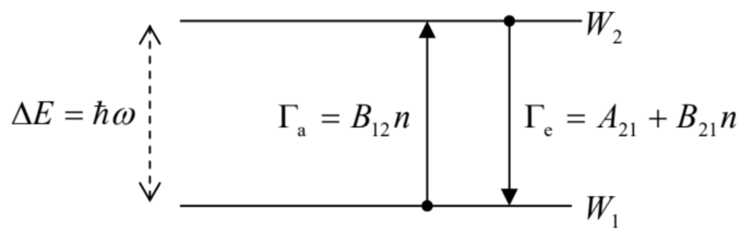Fig. 9.4. The Einstein coefficients on the atomic quantum transition diagram – cf. Fig. 7.6.

I cannot resist the temptation to use this point for a small detour - an alternative derivation of the Bose-Einstein statistics for photons. Indeed, in the thermodynamic equilibrium, the average probability flows between levels 1 and 2 (see Fig. 4 again) should be equal: 30 \[W_{2}\left\langle\Gamma_{\mathrm{e}}\right\rangle=W_{1}\left\langle\Gamma_{\mathrm{a}}\right\rangle,\] where \(W_{1}\) and \(W_{2}\) are the probabilities for the atomic system to occupy the corresponding levels, so that Eqs. (56) and (58) yield \[W_{2} \Gamma_{\mathrm{s}}\langle 1+n\rangle=W_{1} \Gamma_{\mathrm{s}}\langle n\rangle, \quad \text { i.e. } \frac{W_{2}}{W_{1}}=\frac{\langle n\rangle}{\langle n\rangle+1},\] where \(\langle n\rangle\) is the average number of photons in the field causing the interstate transitions. But, on the other hand, for an atomic subsystem only weakly coupled to its electromagnetic environment, we ought to have the Gibbs distribution of these probabilities: \[\frac{W_{2}}{W_{1}}=\frac{\exp \left\{-E_{2} / k_{\mathrm{B}} T\right\}}{\exp \left\{-E_{1} / k_{\mathrm{B}} T\right\}}=\exp \left\{-\frac{\Delta E}{k_{\mathrm{B}} T}\right\}=\exp \left\{-\frac{\hbar \omega}{k_{\mathrm{B}} T}\right\} .\] Requiring Eqs. (61) and (62) to give the same result for the probability ratio, we get the Bose-Einstein distribution for the electromagnetic field in thermal equilibrium: \[\langle n\rangle=\frac{1}{\exp \left\{\hbar \omega / k_{\mathrm{B}} T\right\}-1}\]

• the same result as that obtained in Sec. \(7.1\) by other means - see Eq. (7.26b).

Now returning to the discussion of Eqs. (56) and (58), their very important implication is the possibility to achieve the stimulated emission of coherent radiation using the level occupancy inversion. Indeed, if the ratio \(W_{2} / W_{1}\) is larger than that given by Eq. (62), the net power flow from the atomic system into the electromagnetic field, \[\text { power }=\hbar \omega \times \Gamma_{s}\left[W_{2}(\langle n\rangle+1)-W_{1}\langle n\rangle\right],\] may be positive. The necessary inversion may be produced using several ways, notably by intensive quantum transitions to level 2 from an even higher energy level (which, in turn, is populated, e.g., by absorption of external radiation, usually called pumping, at a higher frequency.)

A less obvious, but crucial feature of the stimulated emission is spelled out by Eq. (55): as was mentioned above, it shows that the final state of the field after the absorption of energy \(\hbar \omega\) from the atom is a pure (coherent) Fock state \((n+1)\). Colloquially, one may say that the new, \((n+1)^{\text {st }}\) photon emitted from the atom is automatically in phase with the \(n\) photons that had been in the field mode initially, i.e. joins them coherently. \({ }^{31}\) The idea of stimulated emission of coherent radiation using population inversion \(^{32}\) was first implemented in the early 1950s in the microwave range (masers) and in 1960 in the optical range (lasers). Nowadays, lasers are ubiquitous components of almost all high-tech systems and constitute one of the cornerstones of our technological civilization.

A quantitative discussion of laser operation is well beyond the framework of this course, and I have to refer the reader to special literature, \({ }^{33}\) but still would like to briefly mention two key points:

(i) In a typical laser, each generated electromagnetic field mode is in its Glauber (rather than the Fock) state, so that Eqs. (56) and (58) are applicable only for the \(n\) averaged over the Fock-state decomposition of the Glauber state - see Eq. (5.134).

(ii) Since in a typical laser \(\langle n\rangle \gg>1\), its operation may be well described using quasiclassical theories that use Eq. (64) to describe the electromagnetic energy balance (with the addition of a term describing the energy loss due to field absorption in external components of the laser, including the useful load), plus the equation describing the balance of occupancies \(W_{1,2}\) due to all interlevel transitions - similar to Eq. (60), but including also the contribution(s) from the particular population inversion mechanism used in the laser. At this approach, the role of quantum mechanics in laser science is essentially reduced to the calculation of the parameter \(\Gamma_{\mathrm{s}}\) for the particular system.

This role becomes more prominent when one needs to describe fluctuations of the laser field. Here two approaches are possible, following the two options discussed in Chapter 7 . If the fluctuations are relatively small, one can linearize the Heisenberg equations of motion of the field oscillator operators near their stationary-lasing "values", with the Langevin "forces" (also time-dependent operators) describing the fluctuation sources, and use these Heisenberg-Langevin equations to calculate the radiation fluctuations, just as was described in Sec. 7.5. On the other hand, near the lasing threshold, the field fluctuations are relatively large, smearing the phase transition between the no-lasing and lasing states. Here the linearization is not an option, but one can use the density-matrix approach described in Sec. 7.6, for the fluctuation analysis. \({ }^{34}\) Note that while the laser fluctuations may look like a peripheral issue, pioneering research in that field has led to the development of the general theory of open quantum systems, which was discussed in Chapter 7 .

---

\({ }^{21}\) Here the sum over all electromagnetic field modes \(j\) may be smuggled back. Since in the quasi-static approximation \(k_{j} a<<1\), which is necessary for the interaction representation by Eq. (24), the matrix elements in Eq. (48) are virtually independent on the direction of the wave vectors, and their magnitudes are fixed by \(\omega\), the summation is reduced to the calculation of the total \(\rho_{\mathrm{f}}\) for all modes, and the averaging of \(e^{2}(\mathbf{r})-\) see below.

\({ }^{22}\) If the same atom is placed into a high- \(Q\) resonant cavity (see, e.g., EM 7.9), the rate of its photon emission is strongly suppressed at frequencies between the cavity resonances (where \(\rho_{\mathrm{f}} \rightarrow 0\) ) - see, e.g., the review by \(\mathrm{S}\). Haroche and D. Klepner, Phys. Today \(\mathbf{4 2 ,} 24\) (Jan. 1989). On the other hand, the emission is strongly (by a factor \(\sim\left(\lambda^{3} / V\right) Q\), where \(V\) is cavity’s volume) enhanced at resonance frequencies - the so-called Purcell effect, discovered by E. Purcell in the 1940s. For a brief discussion of this and other quantum electrodynamic effects in cavities, see the next section.

\({ }^{23}\) This was the breakthrough result obtained by P. Dirac in 1927, which jumpstarted the whole field of quantum electrodynamics. An equivalent expression was obtained from more formal arguments in 1930 by V. Weisskopf and E. Wigner, so that sometimes Eq. (53) is (very unfairly) called the "Weisskopf-Wigner formula".

\({ }^{24}\) See, e.g., EM Sec. 8.2, in particular Eq. (8.29).

\({ }^{25}\) The scale \(c \tau\) of the spatial extension of the corresponding wave packet is surprisingly macroscopic - in the range of a few millimeters. Such a "human" size of spontaneously emitted photons makes the usual optical table, with its \(1-\mathrm{cm}\)-scale components, the key equipment for many optical experiments - see, e.g., Fig. \(2 .\)

\({ }^{26}\) As was already discussed in Sec. 5.6, for a single spin-less particle moving in a spherically-symmetric potential (e.g., a hydrogen-like atom), the orbital selection rules are simple: the only allowed electric-dipole transitions are those with \(\Delta l \equiv l_{\mathrm{fin}}-l_{\mathrm{ini}}=\pm 1\) and \(\Delta m \equiv m_{\mathrm{fin}-} m_{\mathrm{ini}}=0\) or \(\pm 1\). The simplest example of the transition that does \(n o t\) satisfy this rule, i.e. is "forbidden", is that between the \(s\)-states \((l=0)\) with \(n=2\) and \(n=1\); because of that, the lifetime of the lowest excited \(s\)-state of a hydrogen atom is as long as \(\sim 0.15 \mathrm{~s}\).

\({ }^{27}\) See, e.g., EM Sec. 8.9.

\({ }^{28}\) Note, however, a major difference between the rate \(\Gamma\) discussed in \(\operatorname{Sec} .2\), and \(\Gamma_{\mathrm{a}}\) in Eq. (57). In our current case, the atomic transition is still between two discrete energy levels (see Fig. 4 below), so that the rate \(\Gamma_{\mathrm{a}}\) is proportional to \(\rho_{\mathrm{f}}\), the density of final states of the electromagnetic field, i.e. the same density as in Eq. (48) and beyond, while the rate (27) is proportional to \(\rho_{\mathrm{a}}\), the density of final (ionized) states of the "trigger" atom-more exactly, of it’s the electron released at its ionization.

\({ }^{29}\) These relations were conjectured, from very general arguments, by Albert Einstein as early as \(1916 .\)

\({ }^{30}\) This is just a particular embodiment of the detailed balance equation (7.198).

\({ }^{31}\) It is straightforward to show that this fact is also true if the field is initially in the Glauber state - which is more typical for modes in practical lasers.

\({ }^{32}\) This idea may be traced back at least to an obscure 1939 publication by V. Fabrikant.

\({ }^{33}\) I can recommend, for example, P. Milloni and J. Eberly, Laser Physics, \(2^{\text {nd }}\) ed., Wiley, 2010, and a less technical text by A. Yariv, Quantum Electronics, 3rd ed., Wiley, \(1989 .\)

\({ }^{34}\) This path has been developed (also in the mid-1960s), by several researchers, notably including M. Sully and W. Lamb - see, e.g., M. Sargent III, M. Scully, and W. Lamb, Jr., Laser Physics, Westview, \(1977 .\)