9.4: Cavity QED

Now I have to visit, at least in passing, the field of cavity quantum electrodynamics (usually called cavity \(Q E D\) for short) - the art and science of creating and using the entanglement between quantum states of an atomic system (either an atom, or an ion, or a molecule, etc.) and the electromagnetic field in a macroscopic volume called the resonant cavity (or just "resonator", or just "cavity"). This field is very popular nowadays, especially in the context of the quantum computation and communication research discussed in Sec. 8.5. \({ }^{35}\)

The discussion in the previous section was based on the implicit assumption that the energy spectrum of the electromagnetic field interacting with an atomic subsystem is essentially continuous, so that its final state is spread among many field modes, effectively losing its coherence with the quantum state of the atomic subsystem. This assumption has justified using the quantum-mechanical Golden Rule for the calculation of the spontaneous and stimulated transition rates. However, the assumption becomes invalid if the electromagnetic field is contained inside a relatively small volume, with its linear size comparable with the radiation wavelength. If the walls of such a cavity mostly reflect, rather than absorb, radiation, then the \(0^{\text {th }}\) approximation the energy dissipation may be disregarded, and the particular solutions \(\mathbf{e}_{j}(\mathbf{r})\) of the Helmholtz equation (5) correspond to discrete, well-separated mode wave numbers \(k_{j}\) and hence well-separated frequencies \(\omega_{j} \cdot{ }^{36}\) Due to the energy conservation, an atomic transition corresponding to energy \(\Delta E=\left|E_{\text {ini }}-E_{\text {fin }}\right|\) may be effective only if the corresponding quantum transition frequency \(\Omega \equiv \Delta E / \hbar\) is close to one of these resonance frequencies. \({ }^{37}\) As a result of such resonant interaction, the quantum states of the atomic system and the resonant electromagnetic mode may become entangled.

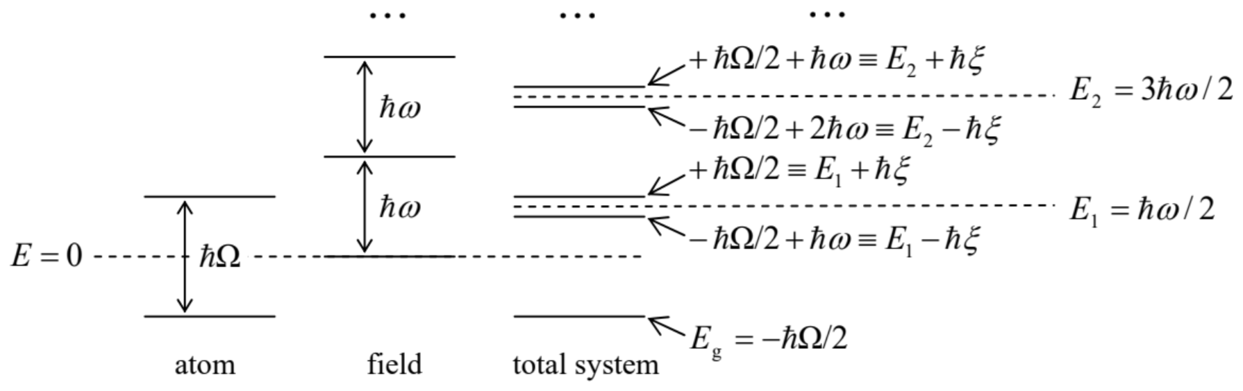
A very popular approximation for the quantitative description of this effect is the so-called \(R a b i\) model, \({ }^{38}\) in which the atom is treated as a two-level system interacting with a single electromagnetic field mode of the resonant cavity. (As was shown in Sec. \(6.5\), this model is justified, e.g., if transitions between all other energy level pairs have considerably different frequencies.) As the reader knows well from Chapters 4-6 (see in particular Sec. 5.1), any two-level system may be described, just as a spin- \(1 / 2\), by the Hamiltonian \(b \hat{I}+\mathbf{c} \cdot \hat{\boldsymbol{\sigma}}\). Since we may always select the energy origin that \(b=0\), and the state basis in which \(\mathbf{c}=c \mathbf{n}_{z}\), the Hamiltonian of the atomic subsystem may be taken in the diagonal form \[\hat{H}_{\mathrm{a}}=c \hat{\sigma}_{z} \equiv \frac{\hbar \Omega}{2} \hat{\sigma}_{z},\] where \(\hbar \Omega \equiv 2 c=\Delta E\) is the difference between the energy levels in the absence of interaction with the field. Next, according to Eq. (17), ignoring the constant ground-state energy \(\hbar \omega / 2\) (which may be always added to the energy at the end - if necessary), the contribution of a single field mode of frequency \(\omega\) to the total Hamiltonian of the system is \[\hat{H}_{\mathrm{f}}=\hbar \omega \hat{a}^{\dagger} \hat{a} \text {. }\] Finally, according to Eq. (16a), the electric field of the mode may be represented as \[\hat{\mathscr{E}}(\mathbf{r}, t)=\frac{1}{i}\left(\frac{\hbar \omega}{2}\right)^{1 / 2} \mathbf{e}(\mathbf{r})\left(\hat{a}-\hat{a}^{\dagger}\right),\] so that in the electric-dipole approximation (24), the cavity-atom interaction may be represented as a product of the field by some (say, \(y\)-) Cartesian component \({ }^{39}\) of the Pauli spin- \(1 / 2\) operator: \[\hat{H}_{\mathrm{int}}=\mathrm{const} \times \hat{\sigma}_{y} \times \mathscr{E}=\mathrm{const} \times \hat{\sigma}_{y} \times\left(\frac{\hbar \omega}{2}\right)^{1 / 2} \frac{1}{i}\left(\hat{a}-\hat{a}^{\dagger}\right)=i \hbar \kappa \hat{\sigma}_{y}\left(\hat{a}-\hat{a}^{\dagger}\right),\] where \(\kappa\) is a coupling constant (with the dimension of frequency). The sum of these three terms, \[\hat{H} \equiv \hat{H}_{\mathrm{a}}+\hat{H}_{\mathrm{f}}+\hat{H}_{\mathrm{int}}=\frac{\hbar \Omega}{2} \hat{\sigma}_{z}+\hbar \omega \hat{a}^{\dagger} \hat{a}+i \hbar \kappa \hat{\sigma}_{y}\left(\hat{a}-\hat{a}^{\dagger}\right) .\] giving a very reasonable description of the system, is called the Rabi Hamiltonian. Despite its apparent simplicity, using this Hamiltonian for calculations is not that straightforward. \({ }^{40}\) Only in the case when the electromagnetic field is large and hence may be treated classically, the results following from Eq. (69) are reduced to Eqs. (6.94) describing, in particular, the Rabi oscillations discussed in Sec. 6.3.The situation becomes simpler in the most important case when the frequencies \(\Omega\) and \(\omega\) are very close, enabling an effective interaction between the cavity field and the atom even if the coupling constant \(\kappa\) is relatively small. Indeed, if both the \(\kappa\) and the so-called detuning (defined similarly to the parameter \(\Delta\) used in Sec. 6.5), \[\xi \equiv \Omega-\omega\] are much smaller than \(\Omega \approx \omega\), the Rabi Hamiltonian may be simplified using the rotating-wave approximation, already used several times in this course. For this, it is convenient to use the spin ladder operators, defined absolutely similarly for those of the orbital angular momentum - see Eqs. (5.153): \[\hat{\sigma}_{\pm} \equiv \hat{\sigma}_{x} \pm i \hat{\sigma}_{y}, \quad \text { so that } \hat{\sigma}_{y}=\frac{\hat{\sigma}_{+}-\hat{\sigma}_{-}}{2 i} .\] From Eq. (4.105), it is very easy to find the matrices of these operators in the standard \(z\)-basis, \[\sigma_{+}=\left(\begin{array}{ll} 0 & 2 \\ 0 & 0 \end{array}\right), \quad \sigma_{-}=\left(\begin{array}{ll} 0 & 0 \\ 2 & 0 \end{array}\right),\] and their commutation rules - which turn out to be naturally similar to Eqs. (5.154): \[\left[\hat{\sigma}_{+}, \hat{\sigma}_{-}\right]=4 \hat{\sigma}_{z}, \quad\left[\hat{\sigma}_{z}, \hat{\sigma}_{\pm}\right]=\pm 2 \hat{\sigma}_{\pm} .\] In this notation, the Rabi Hamiltonian becomes \[\hat{H}=\frac{\hbar \Omega}{2} \hat{\sigma}_{z}+\hbar \omega \hat{a}^{\dagger} \hat{a}+\frac{\hbar \kappa}{2}\left(\hat{\sigma}_{+}-\hat{\sigma}_{-}\right)\left(\hat{a}-\hat{a}^{\dagger}\right),\] and it is straightforward to use Eq. (4.199) and (73) to derive the Heisenberg-picture equations of motion for the involved operators. (Doing this, we have to remember that operators of the "spin" subsystem, on one hand, and of the field mode, on the other hand, are defined in different Hilbert spaces and hence commute - at least at coinciding time moments.) The result (so far, exact!) is \[\begin{gathered} \dot{\hat{a}}=-i \omega \hat{a}+\frac{i \kappa}{2}\left(\hat{\sigma}_{+}-\hat{\sigma}_{-}\right), \quad \dot{\hat{a}}^{\dagger}=i \omega \hat{a}^{\dagger}+\frac{i \kappa}{2}\left(\hat{\sigma}_{+}-\hat{\sigma}_{-}\right) \\ \dot{\hat{\sigma}}_{\pm}=\pm i \Omega \hat{\sigma}_{\pm}+2 i \kappa\left(\hat{a}-\hat{a}^{\dagger}\right) \hat{\sigma}_{z}, \quad \dot{\hat{\sigma}}_{z}=i \kappa\left(\hat{a}^{\dagger}-\hat{a}\right)\left(\hat{\sigma}_{+}+\hat{\sigma}_{-}\right) \end{gathered}\] At negligible coupling, \(\kappa \rightarrow 0\), these equations have simple solutions, \[\hat{a}(t) \propto e^{-i \omega t}, \quad \hat{a}^{\dagger}(t) \propto e^{i \omega t}, \quad \hat{\sigma}_{\pm}(t) \propto e^{\pm i \Omega t}, \quad \hat{\sigma}_{z}(t) \approx \text { const },\] and the small terms proportional to \(\kappa\) on the right-hand sides of Eqs. (75) cannot affect these time evolution laws dramatically even if \(\kappa\) is not exactly zero. Of those terms, ones with frequencies close to the "basic" frequency of each variable would act in resonance and hence may have a substantial impact on the system’s dynamics, while non-resonant terms may be ignored. In this rotating-wave approximation, Eqs. (75) are reduced to a much simpler system of equations: \[\begin{gathered} \dot{\hat{a}}=-i \omega \hat{a}-\frac{i \kappa}{2} \hat{\sigma}_{-}, \quad \dot{\hat{a}}^{\dagger}=i \omega \hat{a}^{\dagger}+\frac{i \kappa}{2} \hat{\sigma}_{+}, \\ \dot{\hat{\sigma}}_{+}=i \Omega \hat{\sigma}_{+}+2 i \kappa \hat{a}^{\dagger} \hat{\sigma}_{z}, \quad \dot{\hat{\sigma}}_{-}=-i \Omega \hat{\sigma}_{-}-2 i \kappa \hat{a} \hat{\sigma}_{z}, \quad \dot{\hat{\sigma}}_{z}=i \kappa\left(\hat{a}^{\dagger} \hat{\sigma}_{-}-\hat{a} \hat{\sigma}_{+}\right) . \end{gathered}\] Alternatively, these equations of motion may be obtained exactly from the Rabi Hamiltonian (74), if it is preliminary cleared of the terms proportional to \(\hat{\sigma}_{+} \hat{a}^{\dagger}\) and \(\hat{\sigma}_{-} \hat{a}\), that oscillate fast and hence self-average to produce virtually zero effect: \[\hat{H}=\frac{\hbar \Omega}{2} \hat{\sigma}_{z}+\hbar \omega \hat{a}^{\dagger} \hat{a}+\frac{\hbar \kappa}{2}\left(\hat{\sigma}_{+} \hat{a}+\hat{\sigma}_{-} \hat{a}^{\dagger}\right), \quad \text { at } \kappa,|\xi|<<\omega, \Omega\] This is the famous Jaynes-Cummings Hamiltonian \({ }^{41}\) which is basic model used in the cavity QED and its applications. \({ }^{42}\) To find its eigenstates and eigenenergies, let us note that at negligible interaction \((\kappa\) \(\rightarrow 0)\), the spectrum of the total energy \(E\) of the system, which in this limit is the sum of two independent contributions from the atomic and cavity-field subsystems, \[\left.E\right|_{\kappa=0}=\pm \frac{\hbar \Omega}{2}+\hbar \omega n \equiv E_{n} \pm \frac{\hbar \xi}{2}, \quad \text { with } n=1,2, \ldots,\] consists \(^{43}\) of close level pairs (Fig. 5) centered to values \[E_{n} \equiv \hbar \omega\left(n-\frac{1}{2}\right) .\] (At the exact resonance \(\omega=\Omega\), i.e. at \(\xi=0\), each pair merges into one double-degenerate level \(E_{n}\).) Since at \(\kappa \rightarrow 0\) the two subsystems do not interact, the eigenstates corresponding to the sublevels of the \(n^{\text {th }}\) pair may be represented by direct products of their independent state vectors: \[|+\rangle \equiv|\uparrow\rangle \otimes|n-1\rangle \quad \text { and }|-\rangle \equiv|\downarrow\rangle \otimes|n\rangle,\] where the first ket of each product represents the state of the two-level (spin-1/2-like) atomic subsystem, and the second ket, that of the field oscillator.

Fig. 9.5. The energy spectrum (79) of the Jaynes-Cummings Hamiltonian in the limit \(\kappa<<|\xi|\). Note again that the energy is referred to the ground-state energy \(\hbar \omega / 2\) of the cavity field.

As we know from Chapter 6 , even weak interaction may lead to strong coherent mixing 44 of quantum states with close energies (in this case, the two states (81) within each pair with the same \(n\) ), while their mixing with the states with farther energies is still negligible. Hence, at \(0<\kappa,|\xi|<<\omega \approx \Omega\), a good approximation of the eigenstate with \(E \approx E_{n}\) is given by a linear superposition of the states (81): \[\left|\alpha_{n}\right\rangle=c_{+}|+\rangle+c_{-}|-\rangle \equiv c_{+}|\uparrow\rangle \otimes|n-1\rangle+c_{-}|\downarrow\rangle \otimes|n\rangle,\] with certain \(c\)-number coefficients \(c_{\pm}\). This relation describes the entanglement of the atomic eigenstates \(\uparrow\) and \(\downarrow\) with the Fock states number \(n\) and \(n-1\) of the field mode. Let me leave the (straightforward) calculation of the coefficients \(\left(c_{\pm}\right)^{\pm}\)for each of two entangled states (for each \(n\) ) for the reader’s exercise. (The result for the corresponding two eigenenergies \(\left(E_{n}\right)_{\pm}\)may be again represented by the same anticrossing diagram as shown in Figs. \(2.29\) and 5.1, now with the detuning \(\xi\) as the argument.) This calculation shows, in particular, that at \(\xi=0\) (i.e. at \(\omega=\Omega),\left|c_{+}\right|=\left|c_{-}\right|=1 / \sqrt{2}\) for both states of the pair. This fact may be interpreted as a (coherent!) equal sharing of an energy quantum \(\hbar \omega=\hbar \Omega\) by the atom and the cavity field at the exact resonance.

As a (hopefully, self-evident) by-product of the calculation of \(c_{\pm}\)is the fact that the dynamics of the state \(\alpha_{n}\) described by Eq. (82), is similar to that of the generic two-level system that was repeatedly discussed in this course - the first time in Sec. \(2.6\) and then in Chapters 4-6. In particular, if the composite system had been initially prepared to be in one component state, for example \(|\uparrow\rangle \otimes|0\rangle\) (i.e. with the atom excited, while the cavity in its ground state), and then allowed to evolve on its own, after some time interval \(\Delta t \sim 1 / \kappa\) it may be found definitely in the counterpart state \(|\downarrow\rangle \otimes|1\rangle\), including the first excited Fock state \(n=1\) of the field mode. If the process is allowed to continue, after the equal time interval \(\Delta t\), the system returns to the initial state \(|\uparrow\rangle \otimes|0\rangle\), etc. This most striking prediction of the JaynesCummings model was directly observed, by G. Rempe et al., only in 1987, although less directly this model was repeatedly confirmed by numerous experiments carried out in the 1960s and 1970s.

This quantized version of the Rabi oscillations can only persist in time if the inevitable electromagnetic energy losses (not described by the basic Jaynes-Cummings Hamiltonian) are somehow compensated - for example, by passing a beam of particles, externally excited into the higher-energy state \(\uparrow\), though the cavity. If the losses become higher, the dissipation suppresses quantum coherence, in our case the coherence between two components of each pair (82), as was discussed in Chapter 7. As a result, the transition from the higher-energy atomic state \(\uparrow\) to the lower-energy state \(\downarrow\), giving energy \(\hbar \omega\) to the cavity \((n-1 \rightarrow n)\), which is then rapidly drained into the environment, becomes incoherent, so that the system’s dynamics is reduced to the Purcell effect, already mentioned in Sec. 3. A quantitative analysis of this effect is left for the reader’s exercise.

The number of interesting physics games one can play with such systems - say by adding external sources of radiation at a frequency close to \(\omega\) and \(\Omega\), in particular with manipulated timedependent amplitude and/or phase, is always unlimited. \({ }^{45}\) Unfortunately, my time/space allowance for the cavity QED is over, and for further discussion, I have to refer the interested reader to special literature. \({ }^{46}\)

---

\({ }^{35}\) This popularity was demonstrated, for example, by the award of the 2012 Nobel Prize in Physics to cavity QED experimentalists S. Haroche and D. Wineland.

\({ }^{36}\) The calculation of such modes and corresponding frequencies for several simple cavity geometries was the subject of EM Sec. \(7.8\) of this series.

\({ }^{37}\) On the contrary, if \(\Omega\) is far from any \(\omega\), the interaction is suppressed; in particular, the spontaneous emission rate may be much lower than that given by Eq. (53) - so that this result is not as fundamental as it may look.

\({ }^{38}\) After the pioneering work by I. Rabi in 1936-37.

\({ }^{39}\) The exact component is not important for final results, while intermediate formulas simplify if the interaction is proportional to either pure \(\hat{\sigma}_{x}\) or pure \(\hat{\sigma}_{y}\).

\({ }^{40}\) For example, an exact quasi-analytical expression for its eigenenergies (as zeros of a Taylor series in the parameter \(\kappa\), with coefficients determined by a recurrence relation) was found only recently - see D. Braak, Phys. Rev. Lett. 107, 100401 (2011).

\({ }^{41}\) It was first proposed and analyzed in 1963 by two engineers, Edwin Jaynes and Fred Cummings, in a Proc. IEEE publication, and it took the physics community a while to recognize and acknowledge the fundamental importance of that work.

\({ }_{42}\) For most applications, the baseline Hamiltonian (78) has to be augmented by additional term(s) describing, for example, the incoming radiation and/or the system’s coupling to the environment, for example, due to the electromagnetic energy loss in a finite- \(Q\)-factor cavity - see Eq. (7.68).

\({ }^{43}\) Only the ground state level \(E_{\mathrm{g}}=-\hbar \Omega / 2\) is non-degenerate \(-\) see Fig. 5.

\({ }^{44}\) In some fields, especially chemistry, such mixing is frequently called hybridization.

\({ }^{45}\) Most of them may be described by adding new terms to the basic Jaynes-Cummings Hamiltonian (78).

\({ }^{46}\) I can recommend, for example, either C. Gerry and P. Knight, Introductory Quantum Optics, Cambridge U. Press, 2005, or G. Agarwal, Quantum Optics, Cambridge U. Press, \(2012 .\)