
4: Atomic spectra, simple models of atoms


- Last updated
- Oct 30, 2021
- Save as PDF

( \newcommand{\kernel}{\mathrm{null}\,}\)
Quantum mechanics had initially the aim to explain the line spectra of atoms seen in optical spectroscopy. The first successful attempt was the Bohr model based on seemingly "ad hoc" postulates. These postulates are actually consequences of the elegant mathematical treatment of the Coulomb problem based on first principles of quantum mechanics. The appearance of angular momentum in this special case hints to its significance in quantum physics.
The Kepler-Newton problem in classical mechanics, Chapter 3.
Bohr’s postulates and the Bohr model
Quantum mechanics had initially the aim to explain the line spectra of atoms seen in optical spectroscopy. Later on it became a fundamental theory explaining all the microscopic phenomena including molecular-, solid state-, nuclear-, and high energy particle physics.
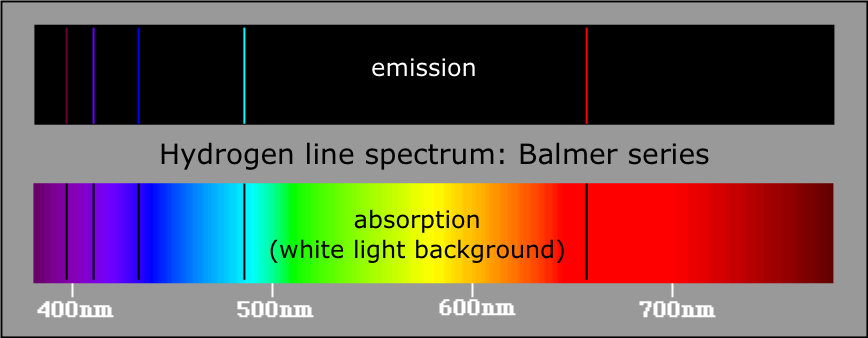
Figure 4.1: Emission and absorption spectra of the Balmer series of hydrogen.
http://www.goiit.com/posts/list/community-shelf-the-bohr-atom-917720.htm
Before going into some details of the quantum mechanical explanation, first we recall how Niels Bohr explained the spectra of atomic gases. He established two postulates.
- Among the classically allowed orbits of the electron moving around the nucleus, there are certain stationary orbits or stationary states with definite energy. The atoms do not radiate if the electron is on such a stationary orbit.
- Electrons can only gain and lose energy by jumping from one allowed orbit with energy E1 to another, with E2 absorbing or emitting electromagnetic radiation with a frequency ν determined by the energy difference of the levels according to the Planck relation:
absorbtion :hν=E2−E1 if E2>E1 emission :hν=E1−E2 if E1>E2 (4.1)
where h is Planck’s constant.
These postulates cannot be understood on the basis of classical physics. An electron moving around the nucleus has a centripetal acceleration, and as all accelerating electric charges it is expected to radiate and lose energy. This would eventually let it fall into the nucleus, so the atom could not be a stable object, which is in sharp contradiction with observations. Therefore the postulates seemed to be "ad hoc". Still they were highly significant, because these statements turned out to be true in view of the "true" quantum mechanics, as well. In that theory, however, these are not fundamental statements but consequences of the deeper general principles and formalism of quantum mechanics.
In addition to these postulates Bohr set up a rule for the H atom how the discrete stationary energies can be obtained again by an ad hoc quantum condition. He prescribed that on these stationary orbits the angular momentum ℓ of the electron orbiting on a circle can have only discrete values, namely an integer multiple of ℏ=h/2π the Planck constant divided by 2π:
L=mvr=nℏ,n=1,2… (4.2)
This is called Bohr’s quantization condition. Combining this with the equation of motion of the electron:
q204πϵ01r2=mv2r (4.3)
i.e. (Coulomb) force equals to mass times (centripetal) acceleration, the total energy of the electron on the circular orbit, of radius r can be calculated from the expression,
E=mv22−q204πϵ01r (4.4)
where the first term is the kinetic energy while the second is the potential energy of the electron in the electric field of the point-like nucleus, one can derive two important results. Introducing the notations
e20=q204πϵ0a0=ℏ2me20 (4.5)
first, the allowed energy values of the stationary states are obtained as
En=−me402ℏ21n2=−e202a01n2n=1,2… (4.6)
Second, the allowed values of the radii of the stationary orbits are:
rn=a0n2 (4.7)
a0 is called the first Bohr radius and its value is a0=0.053nm, and
En=E11n2E1=−2.2aJ=−13.6eV=−1 Rydberg =−1/2hartree (4.8)
The negative sign means that the electron is in a bound state, as the zero level of the potential energy is at r=∞, where the electron becomes free and has zero energy if ν=0. The state with this lowest value of energy is called the ground state of the H atom, and −E1 is the minimal energy to be given to a H atom in order to ionize it, i.e. to strip off the electron from the nucleus. These results were in accordance with the experimental observations of the emission line spectrum of atomic Hydrogen, the different series, etc. with the Rydberg formula (See Figure 4.2).
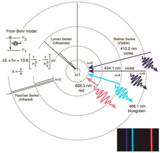
Figure 4.2: Visualization of the emission spectrum lines of atomic Hydrogen.
http://hyperphysics.phy-astr.gsu.edu/hbase/hyde.html
Calculate the wavelengths of the first four Balmer lines which correspond to transitions arriving to the level with n=2. What is the limit of these lines where the continuum begins?
Be, as it is, funny, the results above did turn out to be true, although the premises we started from were definitely wrong. There is a quantization condition for the angular momentum given but in a very different sense than that given in the Bohr model. And this quantization condition is rather a result of the deeper principles of quantum mechanics – explained in section 2 – than an apriori assumption. So this accidental coincidence shows that starting from start premise one can arrive to any result, including the ce correct one. Similar assumption did not lead however to reasonable results in the case of more complicated atoms, and had to be abandoned in the view of quantum mechanics.
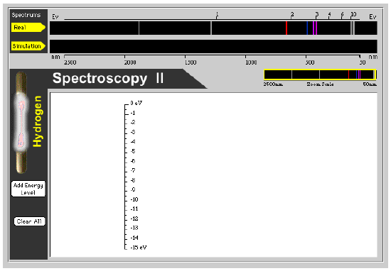
We can investigate the origin of spectral lines in several steps with this interactive shockwave animation.
The radial equation of quantum mechanics
The Schrödinger energy eigenvalue equation for any central field problem, including in particular the Coulomb potential has the form
−ℏ22mΔψ(r)+V(|r|)ψ(r)=εψ(r) (4.9)
where the potential energy depends only on the value |r|=r i.e. on the distance from a centre.
We shall now outline the procedure how the energy eigenvalues and the stationary states can be obtained mathematically, restricting ourselves only to the bound states, that play a very important role in atomic physics, not only in the case of the H atom. In order to find the solution of this equation one introduces spherical coordinates, ψ(r)=ψ(r,θ,ϕ) indicated by the spherical symmetry of the potential. The eigenvalue equation takes the form
−ℏ22m(Δr+1r2Δθϕ)ψ(r,θ,φ)+V(r)ψ(r,θ,φ)=εψ(r,θ,ϕ) (4.10)
where and Δθϕ are the radial and angular parts of the Laplacian, respectively. We separate the radial and angular parts of the wave function with the ansatz (assumption)
ψ(r)=ψ(r,θ,ϕ)=R(r)Ymℓ(θ,ϕ)=u(r)rYmℓ(θ,ϕ) (4.11)
Using the results of the previous section about angular momentum we obtain the following ordinary differential equation for R(r)
−ℏ22m(∂2∂r2+2r∂∂r)R(r)+ℏ212mℓ(ℓ+1)r2R(r)+V(r)R(r)=εR(r) (4.12)
This is called the radial equation, yielding
−ℏ22md2udr2+ℏ22mℓ(ℓ+1)r2u(r)+V(r)u(r)=εu(r) (4.13)
for u(r)=rR(r) which is also called sometimes radial equation.
Show that u(r) obeys the equation (4.13).
The latter form for the unknown u(r) is similar to a one dimensional eigenvalue problem, containing an effective potential V(r)+ℏ22mℓ(ℓ+1)r2, where the last term is a centrifugal potential, appearing also in the corresponding classical problem in the form L2/2mr2.
Asymptotic behaviour of the solutions
Asymptotics in infinity
As we assume that V(∞)→0, then for r→∞ the potential energy and the centrifugal energy are negligible and we obtain the equation
−ℏ22md2udr2=εu (4.14)
We rewrite it as
d2udr2+2mℏ2εu=0 (4.15)
If , corresponding ε≥0, the two solutions are eikr and e−ikr. As we noted earlier these are not square integrable. The corresponding R(r) behave as
R+(r)∼1rei(kr−εt)R−(r)∼1re−i(kr+εt) for r→∞ (4.16)
where time dependence was included in order to see, that R+(r) describes an outgoing spherical wave, an electron with positive total energy that can leave the atom for r→∞. R−(r) is an incoming spherical wave, and both are used for the description of scattering processes, which we do not analyze here.
Square integrable solutions are obtained only if ε<0. Then with the notation:
0<−2mℏ2ε=:κ2 (4.17)
the two appropriate linearly independent solutions of Eq. (4.15) are eκr and e−κr, the first of which is not square integrable on [0,∞) because κ>0. The second solution is proper, as it decays exponentially for r→∞, that is why it will lead to bound state, which is square integrable. Thus we have:
u(r→∞)∼e−κr (4.18)
Asymptotics near the origin
We assume here that the potential energy V(r) remains finite at r=0, or even if it diverges that is not faster than 1/r2. The Coulomb potential belongs to this class, as it is divergent only as 1/r. Then in the radial equation (4.13) the potential energy and εu can be omitted besides the dominant centrifugal term, getting to the second order equation
d2udr2−ℓ(ℓ+1)r2=0 (4.19)
which has a two solutions rℓ+1 and 1/rℓ.
Find the solutions of (4.19) in the form rk.
Show that 1/rℓ is not square integrable on [0,∞), if ℓ>0
According to the solution of the problem above, the solution of the form of 1/rℓ will not be an appropriate one if ℓ>0, and by a little more subtle argumentation it can be shown that this holds true for ℓ=0, as well. This means that we can afford only the nonsingular solution rℓ+1 close to r=0, i.e. the radial part of the wave function around 0 behaves as.
R(r)=u(r)/r∼rℓ (4.20)
i.e it goes to zero if ℓeq0, and remains constant for ℓ=0, ie. for s states.
The radial equation for the bound states can be written with the notation introduced in (4.17)
d2udr2−ℓ(ℓ+1)r2u−2mℏ2V(r)u=−2mℏ2εu=κ2u (4.21)
It will be useful to write the equation in terms of dimensionless variable κr=ϱ:
(d2dϱ2−ℓ(ℓ+1)ϱ2−V(ϱ/κ)|ε|−1)u(ϱ)=0 (4.22)
where the asymptotic conditions require u(ϱ→0)∼ϱℓ+1 and u(ϱ→∞)∼e−ϱ.
This radial equation is often used in atomic physics, a solution in a closed analytic form can be obtained only if the potential V(r) has certain special forms. Therefore one usually applies numerical methods for the solutions. For one of the most important cases: the 1/r Coulomb type potential the solutions can be expressed in terms of elementary analytic functions. The next section deals with this problem.
Eigenvalue problem of the Coulomb potential
In the case of the attractive Coulomb field the radial equation will be written for the more general case of Hydrogen-like ions, where the number of protons in the nucleus is Z≥1, which bound a single electron. Examples are the singly ionized Helium: He+(Z=2), doubly ionized Lithium Li++(Z=3), etc. The potential energy is then V(r)=−Ze20r, where the notation of Eq. (4.5) is used. With κr=ϱ, V(ϱ/κ)=−Ze20κϱ, and the third term in the radial equation is V(ϱ/κ)|ε|=−2mZe20ℏ2κ1ϱ=−ϱ0ϱ. where we have introduced the notation:
ϱ0=2mZe20ℏ2κ=2Zκa0 (4.1)
The radial equation itself takes the form:
(d2dϱ2−ℓ(ℓ+1)ϱ2+ϱ0ϱ−1)u(ϱ)=0 (4.2)
According to the asymptotic conditions obtained in the previous subsection we seek the solution as
u(ϱ)=ϱℓ+1w(ϱ)e−ϱ (4.3)
where the factor ϱℓ+1 takes care about the proper behaviour close to zero, the factor e−ϱ at infinity, and w(ϱ) – which is to be determined – should ensure that this form of u(ϱ) is the exact solution of equation (4.2). Putting the expression of uu given by (4.3) into (4.2), we obtain the differential equation:
ϱd2wdϱ2+2(ℓ+1−ϱ)dwdϱ+(ϱ0−2(ℓ+1))w=0 (4.4)
The solution of the equation for w(ϱ) must not vitiate the prescribed asymptotic forms stipulated by (4.3), which means that w(ϱ) must have a power series (with positive exponents) around zero, and for ϱ→∞ it must grow slower than eϱ in order to maintain the condition u(ϱ→∞)∼e−ϱ If one looks for a solution
w(ϱ)=∑∞k=0akϱk (4.5)
and substitutes it into (4.4), one obtains a recurrence relation between the coefficients :
ak+1=2(k+ℓ+1)−ϱ0(k+1)(k+2ℓ+2)ak (4.6)
In addition it can be shown that if the series (4.5) were infinite, the recurrence relation would behave as the one of the power series of e2ϱ which would mean that the asymptotic condition u(ϱ→∞)∼e−ϱ would be replaced by u(ϱ→∞)∼eϱ which was not allowed, as we required square integrability. Therefore the sum in (4.5) must remain finite. This means that there exist an integer nr, for which anreq0, but anr+1=0, and then, as it follows from (4.6), all ak=0, for k>nr. In other words the sum giving w(ϱ) must reduce to a polynomial of degree nr. This is possible, if and only if the nominator of the coefficient of anr given by the right hand side of of (4.6) vanishes, thus:
ϱ0=2(nr+ℓ+1) (4.7)
The degree nr of the polynomial w is called as radial quantum number. Now one introduces the principal quantum number with the definition
n:=nr+ℓ+1 (4.8)
which is a positive integer. The name principal is given to it, because this is the quantum number that determines the energy eigenvalues. (This statement will be refined later). In order to see this we recall the notation introduced in (4.1)
ϱ0=2mZe20ℏ2κ=2Zκa0=2n (4.9)
and we get κn=Zna0=2mZe20ℏ2n. From the definition of κ, namely ε=−ℏ2κ22m the eigenvalues corresponding to the Coulomb potential are the following:
εn=−mZ2e402ℏ21n2=−Ze202a01n2,n=1,2… (4.10)
This is the most important result: it turns out that the energy eigenvalue equation has square integrable solutions only if ε<0, and in addition only if ε equals to certain discrete numbers, which are equal to those obtained by Bohr from his (erroneous) quantization condition.
The energy eigenvalues of this discrete spectrum are called the bound state energies of the Coulomb potential.
The eigenvalues agree very well with the experimental values of the primary spectrum of the H atom (Z=1) the Lyman, Balmer etc. series. The result also agrees with the formula obtained from the Bohr model. But the Bohr model works only for the H atom, i.e. for the Coulomb potential, while the quantum mechanical procedure works well with any potential.
With the procedure above, we obtained the discrete spectrum, where the role of the boundary conditions is to be remembered. It is important, however, that there are also solutions with ε>0, where ε can be any nonnegative number. The latter part of the eigenvalues form the continuous spectrum, and the corresponding eigenstates are the scattering states. These functions are not square integrable, but similarly to the the De Broglie waves, continuous superpositions can be formed from them which are in turn square integrable.
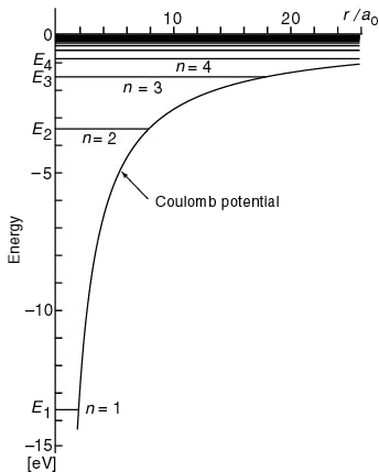
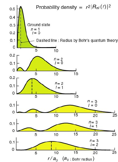
Figure 4.3: On the left you can see the energy diagram of the stationary states of the Hydrogen atom. While on the right figures show the position probability densities of the electron-nucleus densities in the states (r2|Rnℓ(r)|2).
http://www.kutl.kyushu-u.ac.jp/seminar/MicroWorld2_E/2Part3_E/2P32_E/hydrogen_atom_E.htm
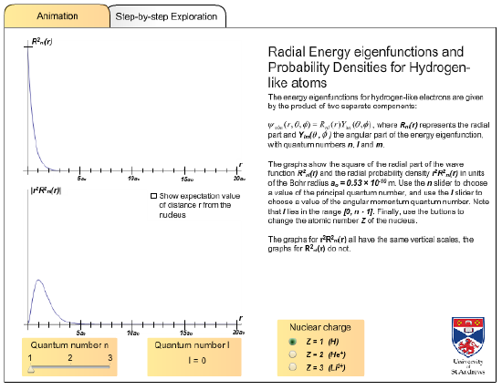
With this flash animation you can investigate the radial eigenfunctions and probability densities (r2|Rnℓ(r)|2) for hydrogen like atoms.
http://www.st-andrews.ac.uk/~qmanim/embed_item_3.php?anim_id=50
The explicit forms of the eigenfunctions can be found in several books, or at the url: http://panda.unm.edu/courses/finley/P262/Hydrogen/WaveFcns.html.
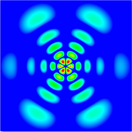
Here you find a presentation on the different possibilities of visualizing the Hydrogen atom.
http://www.hydrogenlab.de/elektronium/HTML/einleitung_hauptseite_uk.html
isit the Grand Orbital Table: http://www.orbitals.com/orb/orbtable.htm, where all atomic orbitals till n=10 are presented.