4.1: Bound States

One of the simplest potentials to study the properties of is the so-called square well potential (Figure $\PageIndex{1}$),

$$V(x) = \left\{\begin{aligned} &0 && | x | > a \\ &-V_0 && | x | < a \end{aligned} \right. \label{4.1}$$

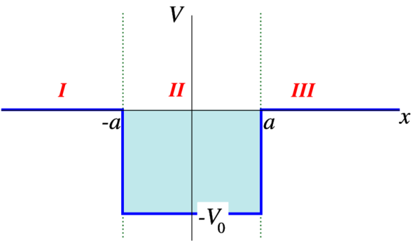
Figure $\PageIndex{1}$: The square well potential

We define three areas, from left to right in Figure $\PageIndex{1}$: I, II and III. In areas I and III we have the Schrödinger equation for a free particle

$$− \dfrac{ℏ^2}{2 m} \dfrac{d^2}{d x^ 2} ψ ( x ) = E ψ ( x ) \label{4.2}$$

whereas in area II we have the equation

$$− \dfrac{ℏ^2}{2 m} \dfrac{d^2}{d x^ 2} ψ ( x ) = ( E + V_0 ) ψ ( x ) \label{4.3}$$

Solution to a few Ordinary Differential Equations

In this class we shall quite often encounter the ordinary differential equations

$$\dfrac{d^2}{d x^2} f( x)=−α^2 f( x) \label{4.4}$$

which has as solution

$$\begin{align} f( x) &= A_1 \cos (α x)+ B_1 \sin (α x) \\[5pt] &= C_1 e^{iα x} + D_1 e^{− iα x}, \label{4.5} \end{align}$$

and

$$\dfrac{d^2}{d x^ 2} g( x)=+α^2 g( x) \label{4.6}$$

which has as solution

$$\begin{align} g( x) &= A_2 \cosh (α x)+ B_2 \sinh (α x) \\[5pt] &= C_2 e^{α x} + D_2 e^{−α x}. \label{4.7} \end{align}$$

Case 1: E> 0

Let us first look at $E> 0$. In that case the equation in regions I and III can be written as

$$\dfrac{d^2}{d x^2} ψ ( x ) = − \dfrac{2 m}{ℏ^2} E ψ ( x ) = − k^2 ψ (x), \label{4.8}$$

where

$$k = \sqrt{ \dfrac{2 m}{ℏ^2}} E \label{4.9}$$

The solution to this equation is a sum of sines and cosines of $k x$, which cannot be normalized: Write

$$ψ_{III}( x)= A \cos ( k x)+ B \sin ( k x)$$

where ($A$ and $B$ can be complex) and calculate the part of the norm originating in region III,

$$\begin{align} \int_a^{∞} |ψ(x)|^2 dx &= \int_a^∞ |A|^2 \cos^2 kx + |B|^2 \sin^2 k x + 2 ℜ ( A B^∗ ) \sin (kx) \cos (kx) dx \\[5pt] &= \lim_{N → ∞} N \int_a^{2 π ∕ k} | A |^2 \cos^2 (kx) + | B |^2 \sin^2 (kx) \\[5pt] &= \lim_{N → ∞} N \left( \dfrac{| A |^ 2}{ 2} + \dfrac{| B |^2}{2} \right ) = ∞ . \label{4.10} \end{align}$$

We also find that the energy cannot be less than $−V_0$, since we cannot construct a solution for that value of the energy. We thus restrict ourselves to $− V_0< E< 0$. We write

$$E = − \dfrac{ ℏ^2}{ k^2 2 m}$$

and

$$E + V_0 = \dfrac{ℏ^2κ^2}{2 m} . \label{4.11}$$

The solutions in the areas I and III are of the form ($i=1,\,3$)

$$ψ ( x ) = A_i e^{k x} + B_i e^{− k x}. \label{4.12}$$

In region II we have the oscillatory solution

$$ψ ( x ) = A_2 \cos ( κ x ) + B_2 \sin ( κ x ). \label{4.13}$$

Now we have to impose the conditions on the wave functions we have discussed before, continuity of $ψ$ and its derivatives. Actually we also have to impose normalisability, which means that $B_1= A_3= 0$ (exponentially growing functions can not be normalized). As we shall see we only have solutions at certain energies. Continuity implies that

$$\begin{align} A_1 e^{ − k a} + B_1 e^{ k a} &= A_2 \cos ( κ a ) − B_2 \sin ( κ a ) \label{4.14A} \\[5pt] A_3 e^{k a} + B_3 e^{− k a} &= A_2 \cos ( κ a ) + B_2 \sin ( κ a ) \label{4.14B} \\[5pt] k A_1 e^{k a} − k B_1 e^{k a} &= κ A_2 \sin ( κ a ) + κ B_2 \cos ( κ a ) \label{4.14C} \\[5pt] k A_3 e^{ k a} − k B_3 e^{− k a} &= − κ A_2 \sin ( κ a ) + κ B_2 \cos ( κ a ) \label{4.14D} \end{align}$$

Tactical Approach

We wish to find a relation between $k$ and $κ$ (why?), removing as maby of the constants $A$ and B. The trick is to first find an equation that only contains $A_2$ and $B_2$. To this end we take the ratio of Equations $\ref{4.14A}$ and $\ref{4.14C}$ and then the ratio of Equations $\ref{4.14B}$ and $\ref{4.14D}$:

$$\begin{align} k &= \dfrac{κ [ A_2 \sin ( κ a ) + B_2 \cos ( κ a ) ]}{ A_2 \cos ( κ a ) − B_2 \sin ( κ a )} \label{4.15A} \\[5pt] k &= \dfrac{κ [ A_2 \sin ( κ a ) − B_2 \cos ( κ a ) ]}{ A_2 \cos ( κ a ) + B_2 \sin ( κ a )} \label{4.15B} \end{align}$$

We can combine Equations $\ref{4.15A}$ and \ref4.15B} to a single one by equating the right-hand sides. After deleting the common factor $κ$, and multiplying with the denominators we find

$$[ A_2 \cos ( κ a ) + B_2 \sin ( κ a ) ] [ A_2 \sin ( κ a ) − B_2 \cos ( κ a ) ] = [ A_2 \sin ( κ a ) + B_2 \cos ( κ a ) ] [ A_2 \cos ( κ a ) − B_2 \sin ( κ a ) ] , \label{4.16}$$

which simplifies to

$$A_2 B_2 = 0 \label{4.17}$$

We thus have two families of solutions, those characterized by $B_2= 0$ and those that have $A_2= 0$.