13.8: Quantum Entanglement

The origins of this story are rooted in the very beginnings of Quantum Mechanics in 1926. A seminal paper was by Einstein, Podolsky and Rosen in 1935, so often the acronym EPR is associated with all this. In the early 1950’s David Bohm re-cast the EPR argument in a clearer form, so sometimes the acronym becomes EPRB. In 1964 John Bell published a theorem that made the situation even clearer, so sometimes we refer to Bell’s Theorem. Finally, the whole story is based on pairs of objects which somehow are interconnected even when they are spatially separated, and we say the objects are entangled.

Bertlmann’s Socks

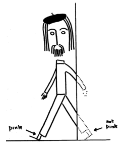
Bertlmann, a colleague of Bell at CERN, always wore mismatched socks. Which color he would have on a given foot on a given day was quite unpredictable. But when you see that the first sock is pink you can be sure that the second sock is not pink, even when you can’t see it. The figure, drawn by Bell, illustrates. There is no mystery here.

An important question for a sock is: “Will it wash?” We imagine a consumer testing organization which wants to determine if a sock will withstand washing when the water is at 0° C, or at 45° C, or at 90° C. We assume, reasonably, that the washability goes down as the temperature increases.

We imagine a large collection of socks. There may be variability in the washability of them. We randomly divide the collection into thirds, and assume that we have a large enough collection that the washability of the socks is equally represented in each third. We wash one collection of socks at 0°, and those that survive we wash at 45°. We wash the second collection of socks at 45°, and those that survive we wash at 90°. We wash the third collection at 0° and those that survive we wash at 90°. Since the washability of each collection of socks is the same:

The number that survive at 0° and not at 45° Plus

The number that survive at 45° and not at 90° Is not less than

The number that survive at 0° and not at 90°

There is no mystery here either. For each member of the third group, either it would not have survived at 45° and would have been in the first group, or it would have survived at 45° and would have been in the second group.

But Bertlmann’s socks come in pairs. We assume that each individual pair of socks has different colours but identical washability. Then if we test a large sample of pairs of his socks the relation at the bottom of the previous page becomes:

The number of pairs in which one survives at 0° and the other not at 45° Plus

The number of pairs in which one survives at 45° and other not at 90° Is not less than

The number of pairs in which one survives at 0° and other not at 90°

Electron Spin

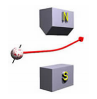
When a charged classical object is spinning, if we throw it between the poles of a weird shaped magnet it will be deflected either up or down. The amount of deflection depends on:

• The total charge on the object and its distribution.
• The rate and orientation of the spin

If we take a beam of electrons from an electron gun and run it through the magnet, we see something strange: all electrons are deflected up by some fixed amount or deflected down by exactly the same amount, and which for each individual electron appears to be random. If the deflection is up, we say the electron is “spin up” and if it is deflected down we say it is “spin down.”

There are substances which emit electrons in pairs. Each electron acts just like the electrons from the electron gun. But when we look at pairs of electrons we see that if one electron is “spin up” then its companion is “spin down” and vice versa. So we can call these Bertlmann’s electrons: if you measure one and see that it is spin up, you know that its companion is not spin up, it is spin down. Physicists often say that these pairs have a total spin of zero and that the two electrons are entangled.

The fact that electrons can have only two spin states is a mystery. The fact that Bertlmann’s electrons have a total spin of zero is not.

There is a further mystery about electrons, either from an electron gun or one of the Bertlmann pairs: if I rotate the magnet by, say, 45° or 90° about the axis of the initial path of the electrons I get the same result as before: all the electrons are deflected up by some fixed amount or deflected down by exactly the same amount, and which for each individual electron appears to be random. Note that the definition of “up” is determined by the orientation of the magnet.

We can extend the washability study for pairs of socks to entangled pairs of electrons with one trivial difference. For the socks if one survived washing at 45° we assumed that the other member of the pair would too. For Bertlmann’s electrons if one is spin up for 45° its companion is spin down for 45°, i.e. its companion is not spin-up for 45°. So now the relation near the top of the previous page becomes:

The number of pairs for which one is spin-up for 0° and the other is spin-up for 45° Plus

The number of pairs for which one is spin-up for 45° and the other is spin-up for 90° Is not less than

The number of pairs for which one is spin-up for 0° and the other is spin-up for 90°

This relation has been experimentally tested, and is not true! So evidently there is some difference between Bertlmann’s socks and Bertlmann’s electrons, and we have made at least one wrong assumption somewhere in deriving this relation for electrons.

It turns out that the actual experimental result is predicted by Quantum Mechanics, so whatever wrong assumptions we made are also violated by that theory.

The Assumptions

We have used some logic in deriving the relation for Bertlmann’s socks and electrons. We also made two assumptions in deriving the relations. Both are so self-evident that it is easy to miss the fact that we made them at all.

First, when we talked about the number of socks or electrons at 0° and 90° we assumed that each would or would not pass the test at 45°. Put another way, we assumed the existence of washability at some temperature or spin at some angle, even if it was not actually measured. Put still another way, we have assumed that there is a reality independent of its observation. This is similar to the old philosophical saw about a tree falling in the forest: if no one is there was there any sound?

Second, when we talk about measuring the washability or spin of one member of a pair to determine something about its companion, we assumed that since we were doing simultaneous measurements of two different socks/electrons at different locations, the effect of one measurement can’t possibly disturb the result of the measurement of the other member of the pair. Put another way, we assumed that no signal or influence can propagate infinitely fast. Sometimes this assumption is called locality.

So experimentally we have proven that at least one of these two assumptions is wrong for entangled electrons.

So What?

The experimental tests have proved that there is no reality separate from its observation and/or different parts of the universe are instantaneously connected to every other part of the universe. So we have learned something profound about the physical world.

Nobody thought more deeply about a universe that does not exist independent of its observation than John Archibald Wheeler. He suggested that we should drop the word “observer” from our vocabulary, replacing it with “participator.” The figure below was devised by him. He comments on the figure:

Symbolic representation of the Universe as a self-excited system brought into being by ‘self-reference’. The universe gives birth to communicating participators. Communicating participators give meaning to the universe … With such a concept goes the endless series of receding reflections one sees in a pair of facing mirrors.

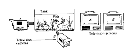
David Bohm thought deeply about a universe which is instantaneously connected to every other part of the universe. He proposed that underlying our everyday universe, which he called the explicate order, there is an underlying order, the implicate, in which there is no separation in space or time. The figure is an analogy devised by Bohm.

We can only look at the television screens, and we see two fish at different locations. As we continue to look, we start noticing a correlation between the motions of the two fish. This is because underlying the reality of the two screens is a single unity, a single fish, that we can only observe from two different perspectives.

So this entanglement business is causing some deep thinking about the nature of the world. A pragmatist might say “So what?” Similarly, in the mid nineteenth century Faraday, Maxwell and others were thinking about the nature of electricity and magnetism. The British prime minister, Gladstone, is reported to have asked Faraday what possible use such idle speculations might have. Faraday replied: “Some day, sir, you will tax it.”

Entanglement almost certainly has practical applications, which presumably will eventually be taxed. These include quantum computers, which may have orders of magnitude more power than any conventional computer can possibly achieve, and quantum teleportation ala the transporter in Star Trek. Developing these applications is a “red hot” field of research and development.

To Learn More

Louisa Gilder, The Age of Entanglement: When Quantum Physics Was Reborn. (2008).

Reading this book caused me to bring Louisa to Toronto for a Physics colloquium in January. The photograph was taken at the colloquium. The colloquium in turn led to an invitation for me to give this talk. The book is available in hardback, paperback, and on Kindle.

John S. Bell, “Bertlmann’s Socks and the Nature of Reality” (1980)

The first few sections of my little document are almost plagiarised1 from Bell’s classic paper. It can easily be found via Google.

N. David Mermin, “Quantum Mysteries for Anyone” (J. Philosophy 78, p. 397, 1981) and “Bringing home the atomic world: Quantum mysteries for anybody” (Amer. J. Physics 49, p. 940, 1981).

These nearly identical papers are brilliant. The first version had a large influence on Louisa Gilder. I have prepared a Flash animation based on Mermin’s papers:

http://faraday.physics.utoronto.ca/P...in/Mermin.html

David Bohm, Wholeness and the Implicate Order (1980).

This book discusses Bohm’s thinking about a non-local universe.

David Harrison, “Bell’s Theorem” (1999, last revision 2006).

A long-winded discussion with some similarities to this document. It is available at:

http://www.upscale.utoronto.ca/PVB/H...lsTheorem.html

I am amazed and pleased that Googling bell’s theorem lists this document 2nd, just after the Wikipedia entry.

 

Author

This document is Copyright © 2010 David M. Harrison. It is licensed under the Creative Commons Attribution-Noncommercial-Share Alike 3.0 license. Basically you are free to share or modify this work for any non-commercial purpose. The details and conditions of the license are at: http://creativecommons.org/licenses/by-nc-sa/3.0/.