13.17: Two analogies to Bell's Theorem
- Page ID
- 5905
\( \newcommand{\vecs}[1]{\overset { \scriptstyle \rightharpoonup} {\mathbf{#1}} } \)
\( \newcommand{\vecd}[1]{\overset{-\!-\!\rightharpoonup}{\vphantom{a}\smash {#1}}} \)
\( \newcommand{\dsum}{\displaystyle\sum\limits} \)
\( \newcommand{\dint}{\displaystyle\int\limits} \)
\( \newcommand{\dlim}{\displaystyle\lim\limits} \)
\( \newcommand{\id}{\mathrm{id}}\) \( \newcommand{\Span}{\mathrm{span}}\)
( \newcommand{\kernel}{\mathrm{null}\,}\) \( \newcommand{\range}{\mathrm{range}\,}\)
\( \newcommand{\RealPart}{\mathrm{Re}}\) \( \newcommand{\ImaginaryPart}{\mathrm{Im}}\)
\( \newcommand{\Argument}{\mathrm{Arg}}\) \( \newcommand{\norm}[1]{\| #1 \|}\)
\( \newcommand{\inner}[2]{\langle #1, #2 \rangle}\)
\( \newcommand{\Span}{\mathrm{span}}\)
\( \newcommand{\id}{\mathrm{id}}\)
\( \newcommand{\Span}{\mathrm{span}}\)
\( \newcommand{\kernel}{\mathrm{null}\,}\)
\( \newcommand{\range}{\mathrm{range}\,}\)
\( \newcommand{\RealPart}{\mathrm{Re}}\)
\( \newcommand{\ImaginaryPart}{\mathrm{Im}}\)
\( \newcommand{\Argument}{\mathrm{Arg}}\)
\( \newcommand{\norm}[1]{\| #1 \|}\)
\( \newcommand{\inner}[2]{\langle #1, #2 \rangle}\)
\( \newcommand{\Span}{\mathrm{span}}\) \( \newcommand{\AA}{\unicode[.8,0]{x212B}}\)
\( \newcommand{\vectorA}[1]{\vec{#1}} % arrow\)
\( \newcommand{\vectorAt}[1]{\vec{\text{#1}}} % arrow\)
\( \newcommand{\vectorB}[1]{\overset { \scriptstyle \rightharpoonup} {\mathbf{#1}} } \)
\( \newcommand{\vectorC}[1]{\textbf{#1}} \)
\( \newcommand{\vectorD}[1]{\overrightarrow{#1}} \)
\( \newcommand{\vectorDt}[1]{\overrightarrow{\text{#1}}} \)
\( \newcommand{\vectE}[1]{\overset{-\!-\!\rightharpoonup}{\vphantom{a}\smash{\mathbf {#1}}}} \)
\( \newcommand{\vecs}[1]{\overset { \scriptstyle \rightharpoonup} {\mathbf{#1}} } \)
\(\newcommand{\longvect}{\overrightarrow}\)
\( \newcommand{\vecd}[1]{\overset{-\!-\!\rightharpoonup}{\vphantom{a}\smash {#1}}} \)
\(\newcommand{\avec}{\mathbf a}\) \(\newcommand{\bvec}{\mathbf b}\) \(\newcommand{\cvec}{\mathbf c}\) \(\newcommand{\dvec}{\mathbf d}\) \(\newcommand{\dtil}{\widetilde{\mathbf d}}\) \(\newcommand{\evec}{\mathbf e}\) \(\newcommand{\fvec}{\mathbf f}\) \(\newcommand{\nvec}{\mathbf n}\) \(\newcommand{\pvec}{\mathbf p}\) \(\newcommand{\qvec}{\mathbf q}\) \(\newcommand{\svec}{\mathbf s}\) \(\newcommand{\tvec}{\mathbf t}\) \(\newcommand{\uvec}{\mathbf u}\) \(\newcommand{\vvec}{\mathbf v}\) \(\newcommand{\wvec}{\mathbf w}\) \(\newcommand{\xvec}{\mathbf x}\) \(\newcommand{\yvec}{\mathbf y}\) \(\newcommand{\zvec}{\mathbf z}\) \(\newcommand{\rvec}{\mathbf r}\) \(\newcommand{\mvec}{\mathbf m}\) \(\newcommand{\zerovec}{\mathbf 0}\) \(\newcommand{\onevec}{\mathbf 1}\) \(\newcommand{\real}{\mathbb R}\) \(\newcommand{\twovec}[2]{\left[\begin{array}{r}#1 \\ #2 \end{array}\right]}\) \(\newcommand{\ctwovec}[2]{\left[\begin{array}{c}#1 \\ #2 \end{array}\right]}\) \(\newcommand{\threevec}[3]{\left[\begin{array}{r}#1 \\ #2 \\ #3 \end{array}\right]}\) \(\newcommand{\cthreevec}[3]{\left[\begin{array}{c}#1 \\ #2 \\ #3 \end{array}\right]}\) \(\newcommand{\fourvec}[4]{\left[\begin{array}{r}#1 \\ #2 \\ #3 \\ #4 \end{array}\right]}\) \(\newcommand{\cfourvec}[4]{\left[\begin{array}{c}#1 \\ #2 \\ #3 \\ #4 \end{array}\right]}\) \(\newcommand{\fivevec}[5]{\left[\begin{array}{r}#1 \\ #2 \\ #3 \\ #4 \\ #5 \\ \end{array}\right]}\) \(\newcommand{\cfivevec}[5]{\left[\begin{array}{c}#1 \\ #2 \\ #3 \\ #4 \\ #5 \\ \end{array}\right]}\) \(\newcommand{\mattwo}[4]{\left[\begin{array}{rr}#1 \amp #2 \\ #3 \amp #4 \\ \end{array}\right]}\) \(\newcommand{\laspan}[1]{\text{Span}\{#1\}}\) \(\newcommand{\bcal}{\cal B}\) \(\newcommand{\ccal}{\cal C}\) \(\newcommand{\scal}{\cal S}\) \(\newcommand{\wcal}{\cal W}\) \(\newcommand{\ecal}{\cal E}\) \(\newcommand{\coords}[2]{\left\{#1\right\}_{#2}}\) \(\newcommand{\gray}[1]{\color{gray}{#1}}\) \(\newcommand{\lgray}[1]{\color{lightgray}{#1}}\) \(\newcommand{\rank}{\operatorname{rank}}\) \(\newcommand{\row}{\text{Row}}\) \(\newcommand{\col}{\text{Col}}\) \(\renewcommand{\row}{\text{Row}}\) \(\newcommand{\nul}{\text{Nul}}\) \(\newcommand{\var}{\text{Var}}\) \(\newcommand{\corr}{\text{corr}}\) \(\newcommand{\len}[1]{\left|#1\right|}\) \(\newcommand{\bbar}{\overline{\bvec}}\) \(\newcommand{\bhat}{\widehat{\bvec}}\) \(\newcommand{\bperp}{\bvec^\perp}\) \(\newcommand{\xhat}{\widehat{\xvec}}\) \(\newcommand{\vhat}{\widehat{\vvec}}\) \(\newcommand{\uhat}{\widehat{\uvec}}\) \(\newcommand{\what}{\widehat{\wvec}}\) \(\newcommand{\Sighat}{\widehat{\Sigma}}\) \(\newcommand{\lt}{<}\) \(\newcommand{\gt}{>}\) \(\newcommand{\amp}{&}\) \(\definecolor{fillinmathshade}{gray}{0.9}\)Background
There are a couple of facts which we will need for our discussion. One is from human biology, and the other from physics.
Issues in the Development of People
The context of our analogy is the nature versus nurture debate about the development of people. Adherents of the nurture position believe that at birth humans are essentially a blank slate, and that their environment as they grow and develop is the only factor that determines characteristics of the individual. Thus matters of choice of profession, mate, musical preferences, morality, etc. are determined by society. Believers in the nature position, on the other hand, say the genetics is crucial in development, and that the characteristics of an individual are determined at birth.
The data are fairly clear that both genetics and environment are approximately equally important in the development of an individual.
One of the types of studies that lead to this conclusion involve identical twins who were separated at birth. Such twins have almost completely identical DNA, and sometimes were raised in very different social environments. Nonetheless, there are often strong correlations between the later behavior of such twins: if one is, say, a firefighter than often the other is also a firefighter. Other characteristics that twins tend to share, even if raised in very different environments, include physical characteristics of their choice of mate, preferences in music, and more.
Later it will be important to note that the correlations are not 100%. Just because one twin is a firefighter does not guarantee that the other is too. Similarly, if one twin really hates the music of Twisted Sister does not guarantee that the other twin will also despise that type of "music." Nonetheless, the correlations are sufficiently strong that it is almost certain that they did not arise by pure chance.
Pairs of Spinning Particles in Physics
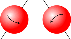
| Most elementary particles, such as electrons, photons, etc., have an intrinsic angular momentum which is usually called spin. For our purposes, we can imagine the particle as a small ball that is spinning about some axis. It turns out that the spin of an electron has only two states, which we call up and down. The origins of this terminology are not important for our purposes here. In the figure, the electron on the left is spin-up and the electron on the right is spin-down. |  |
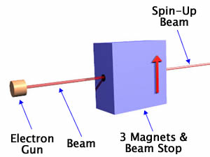
| It is possible to construct a "filter" that selects only spin-up electrons. Again the details of what is in the box are not important for our purposes. What is important here is that one-half of the electrons from the electron gun will emerge from the filter with the same speed in the same direction as before they entered the box, and one-half of the electrons will not emerge. Which is the case for an individual electron is random. You will also want to notice that we have painted an arrow on the side of the box to indicate what direction is up. |  |
| The apparatus actually defines the direction of up. If we rotate it by some angle, again one-half of the incident electrons emerge from the filter, and which is the case for an individual electron is random. |
|
There are some radioactive materials for which when an individual atom decays it simultaneously emits two electrons in opposite directions. These pairs of electrons have a total spin of zero: if one electron is spin-up, its companion electron is spin-down and vice versa. Such pairs of particles are called entangled quantum pairs.
The Analogy
We shall begin by assuming that the nurture position on human development is correct. This assumption means that we would expect that for identical twins separated at birth, any later correlations in their choices of profession, mate, etc. are due to similarities in the environment in which the twins were raised. Each twin's environment is local to the separate individual, and we are assuming that this local environment causes the later behavior of the individual. In Physics-speak, we call this assumption local causality.
There are two kinds of correlation experiments that we can do.
- Correlations in the choice of profession, or the taste in music, or some other characteristic.
- Correlations of the choice of profession of one twin with the musical taste of the other twin. This is a more sophisticated experiment, and the analysis will require more statistical information.
 The studies of the correlations of twin behavior, then, show that the assumption of local causality is incorrect.
We can also do correlation experiments for the entangled quantum pairs of electrons that we discussed above. The source of the total spin-zero entangled electron pairs is in the center of the figure, and the two electrons from each decay go in opposite directions.
Note that the two filters have opposite orientations.
It turns out that one-half of the electrons traveling to the right pass through its filter and one-half do not, and which is the case for an individual electron is random. Similarly one-half of the electrons traveling to the left pass through its filter and one-half do not, and which is the case for an individual electron is random. However, when we examine the correlations, if the right-hand electron passes through its filter its companion left-hand electron also passes through its filter. If the right-hand electron does not pass through its filter its companion left-hand electron does not pass through its filter. This is a consequence of the fact that the two electrons have a total spin of zero, so if one is spin-up the other is spin-down provided the direction of "up" is the same for both measurements. Here the direction of "up" is opposite for the two filters.
For the identical twins, correlations in the same characteristic such as profession showed that local causality is not true in the nature vs. nurture debate. However, this correlation in electron spins does not violate local causality. This circumstance is more analogous to the following:
We carefully saw a coin in half along its plane, so one piece has the "head" and the other has the "tails." We put each piece in an envelope and walk the two envelopes away from each other. If we open one envelope and see a heads, we are guaranteed that the other piece contains a tails.
 However, when we set the electron filters at orientations other than opposite each other we see strange correlations. To the right we have the right-hand filter oriented at zero degrees, and the left-hand filter tipped by 45 degrees.
In fact, the conflict with local causality for entangled electron spin correlations only shows up when we set the right and left hand filters at different angles. This is analogous the the twin correlation measurements where we try to correlate the profession of one with the musical taste of the other. The actual tests involve orienting the filters at zero degrees, 45 degrees, and 90 degrees.
We explore in more detail how this conflict arises in the next section.
The Second Analogy: More Boxes
A Flash animation that duplicates much of the discussion of this section is available. It requires Flash 6, and has a file size of 78k. You may access it by clicking here. It will appear in a separate window.
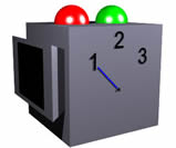
 We imagine a box, such as is shown to the right. Although nobody has every made such a box, there is no reason why it could not be constructed. It has a red and green light on top, and a switch that can be set to three positions: 1, 2, and 3. The apparatus is self contained, and has batteries inside to drive the lights and whatever mechanism is inside.
The box is a detector, and one of the lights will light up when a particle enters it from the left.
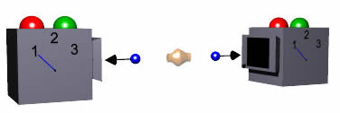
 We have two of these detectors, and place them on either side of some device which emits pairs of particles in opposite directions.
We have bazillions of pairs of these particles go through the detectors, and set the switch positions randomly for each pair. If the boxes are measuring electron spin, then the switches could correspond to orienting the spin filters at zero, 45, and 90 degrees, and the pairs of particles could be entangled electron pairs. Soon we shall attempt to build another more classical model of what is being measured, and will run into trouble with it.
We record which lights flash for each pair and what are the switch positions. There are two cases:
- If both switches on the boxes are set to the the same positions, either 1 or 2 or 3, the same light flashes on both boxes. Either both red lights flash or both green lights flash. Half of the time both red lights flash, the other half of the time both green lights flash.
- If the switches are set to different positions both detectors flash the same color one-quarter of the time, either both red or both green. One half of the time when both colors flash they are both red, the other half of the time they are both green. Three-quarters of the time the detectors flash different colors, either red on the left and green on the right or green on the left and red on the right; in this case each of the two possibilities occur half of the time.
Explaining Case 1
Imagine that when the switch is in position 1 it measures the speed of the object, when it is position 2 it measures the size, and in position 3 it measure the shape of the object.
| Switch Position | Measures | Green Light | Red Light |
|---|---|---|---|
| 1 | Speed | Flashes when particle is going fast | Flashes when particle is going slow |
| 2 | Size | Flashes when particle is big | Flashes when particle is small |
| 3 | Shape | Flashes when the particle is a sphere | Flashes when the particle is not a sphere |
Then the experimental results are easy to explain:
- The pairs of particles always have the same speeds, the same size, and the same shape.
- Half of the time both the particles are moving fast, half of the time both are moving slow.
- Half of the time both the particles are big, half of the time they are both small.
- Half of the time both particles are spheres, half of the time they are not.
- There are eight different states the pairs of particles can be in, each occurring with equal frequency:
- Fast big spheres.
- Slow big spheres.
- Fast little spheres.
- Slow little spheres.
- Fast big non-spheres
- Slow big non-spheres
- Fast little non-spheres.
- Slow little non-spheres.
What About Case 2?
There are six settings of the switches which are different.
For the case of fast big spheres here are the possible switch settings and the results:
| Left Switch | Left Light | Right Switch | Right Light |
|---|---|---|---|
| 1 | Green | 2 | Green |
| 2 | Green | 1 | Green |
| 2 | Green | 3 | Green |
| 3 | Green | 2 | Green |
| 1 | Green | 3 | Green |
| 3 | Green | 1 | Green |
So for this case all the switch settings end up with the both green lights flashing. For slow small non-spheres, similarly, both red lights will flash for all six switch positions. We expect one-quarter of the bazillion pairs of particles to be either fast big spheres or slow small non-spheres. So far so good: the experimental result is that the lights flash the same color one-quarter of the time.
But imagine the case of pairs of fast big non-spheres. Here are the possible switch settings and the results:
| Left Switch | Left Light | Right Switch | Right Light |
|---|---|---|---|
| 1 | Green | 2 | Green |
| 2 | Green | 1 | Green |
| 2 | Green | 3 | Red |
| 3 | Red | 2 | Green |
| 1 | Green | 3 | Red |
| 3 | Red | 1 | Green |
Only two of the six possible settings have both lights flash the same color, green in this case. But the switch settings are made at random, so we expect each of the six possible results in the above table to occur with equal frequency. So both lights flash the same color one-third of the time.
The same argument can be made for the other five pairs that are not big fast spheres or small slow non-spheres: both lights will flash the same color one-third of the time.
Imagine we take data for 24 bazillion pairs of particles. We expect each of the eight possible states of speed, size, and shape to occur with equal frequency, so our sample will have 3 bazillion pairs of each type. We then expect the following results when the switches are set to different positions:
| Type | Number | Number of Pairs For Which the 2 Lights Flash the Same Color | Color | Fraction |
|---|---|---|---|---|
| fast big spheres | 3 bazillion | 3 bazillion | both green | 1 |
| slow big spheres | 3 bazillion | 1 bazillion | both green | 1/3 |
| fast little spheres | 3 bazillion | 1 bazillion | both green | 1/3 |
| slow little spheres | 3 bazillion | 1 bazillion | both red | 1/3 |
| fast big non-spheres | 3 bazillion | 1 bazillion | both green | 1/3 |
| slow big non-spheres | 3 bazillion | 1 bazillion | both red | 1/3 |
| fast little non-spheres | 3 bazillion | 1 bazillion | both red | 1/3 |
| slow little non-spheres | 3 bazillion | 3 bazillion | both red | 1 |
| Total | 24 bazillion | 12 bazillion | half both red, half both green | 1/2 |
So when we summarise the data for all the pairs of particles that we measured, we would not expect to have different colors flashing on the two detectors one-quarter of the time, but instead one-half of the time. But the experimental result is one-quarter, not one-half.
This example has been thinking about classical objects, which is tantamount to assuming local causality. Thus we see that these correlation measurements violate local causality, in exactly the same way the the electron spin measurements of entangled electron pairs violate local causality.
This entire section is a slight simplification of Mermin's analysis, which is listed in the references. I close with the conclusion of that lovely paper:
I shall not describe how contemporary physical theory accounts for the behavior of the device except to note that although, in its own way, the explanation is very simple, it is far from obvious, and, some might argue, hardly an explanation at all. Instead, I only emphasize again that we live in a world where such a device can be built; nature is stranger and more wonderful than we had once thought or could possible [sic] have imagined. Ponder the device a little more if that seems too extreme a conclusion.
Further Study
Here are some documents on particle spin, Bell's Theorem, and the Nature vs. Nurture debate which are accessible to the layperson.
Spin
- A non-mathematical treatment, by the author of this document, is available on the web at:
http://www.upscale.utoronto.ca/PVB/Harrison/SternGerlach/SternGerlach.html (html)
http://www.upscale.utoronto.ca/PVB/Harrison/SternGerlach/SternGerlach.pdf (pdf) - A wonderful discussion which does do a bit of the mathematics is Richard P. Feynman, Robert B. Leighton and Matthew Sands, The Feynman Lectures on Physics, Vol. III, Chapters 5 - 6, ISBN: 0201500647.
Bell's Theorem
- A brilliant example, which is non-mathematical but subtle, is N.D. Mermin, American Journal of Physics 49, 940 (1981). Many institutions, including the University of Toronto, have subscriptions to this journal so they may be accessed from any computer whose IP number corresponds to the subscribing institution. The American Journal of Physics is available on-line at: scitation.aip.org/ajp/
- A clever proof, using simple Venn diagrams, is B. d'Espagnat, Scientific American 241, 158 (November 1979).
- A "chaotic ball" analogy is C.H. Thompson and H. Holstein, Foundations of Physics Letters 9, 357 (1996), http://www.arxiv.org/format/quant-ph/9611037 .
- A mostly non-mathematical treatment, by the author of this document, is available on the web at:
http://www.upscale.utoronto.ca/PVB/Harrison/BellsTheorem/BellsTheorem.html (html)
http://www.upscale.utoronto.ca/PVB/Harrison/BellsTheorem/BellsTheorem.pdf (pdf)
Nature versus Nurture
- Judith Rich Harris, The Nurture Assumption ( Free Press,1999), ISBN: 0684857073
- Steven Pinker, The Blank Slate (Viking, 2002), ISBN: 0670031518
Author
David M. Harrison, Department of Physics, University of Toronto, harrison@physics.utoronto.ca.


