5.4: The Electron-Photon Interaction
- Page ID
- 34662

\( \newcommand{\vecs}[1]{\overset { \scriptstyle \rightharpoonup} {\mathbf{#1}} } \)
\( \newcommand{\vecd}[1]{\overset{-\!-\!\rightharpoonup}{\vphantom{a}\smash {#1}}} \)
\( \newcommand{\dsum}{\displaystyle\sum\limits} \)
\( \newcommand{\dint}{\displaystyle\int\limits} \)
\( \newcommand{\dlim}{\displaystyle\lim\limits} \)
\( \newcommand{\id}{\mathrm{id}}\) \( \newcommand{\Span}{\mathrm{span}}\)
( \newcommand{\kernel}{\mathrm{null}\,}\) \( \newcommand{\range}{\mathrm{range}\,}\)
\( \newcommand{\RealPart}{\mathrm{Re}}\) \( \newcommand{\ImaginaryPart}{\mathrm{Im}}\)
\( \newcommand{\Argument}{\mathrm{Arg}}\) \( \newcommand{\norm}[1]{\| #1 \|}\)
\( \newcommand{\inner}[2]{\langle #1, #2 \rangle}\)
\( \newcommand{\Span}{\mathrm{span}}\)
\( \newcommand{\id}{\mathrm{id}}\)
\( \newcommand{\Span}{\mathrm{span}}\)
\( \newcommand{\kernel}{\mathrm{null}\,}\)
\( \newcommand{\range}{\mathrm{range}\,}\)
\( \newcommand{\RealPart}{\mathrm{Re}}\)
\( \newcommand{\ImaginaryPart}{\mathrm{Im}}\)
\( \newcommand{\Argument}{\mathrm{Arg}}\)
\( \newcommand{\norm}[1]{\| #1 \|}\)
\( \newcommand{\inner}[2]{\langle #1, #2 \rangle}\)
\( \newcommand{\Span}{\mathrm{span}}\) \( \newcommand{\AA}{\unicode[.8,0]{x212B}}\)
\( \newcommand{\vectorA}[1]{\vec{#1}} % arrow\)
\( \newcommand{\vectorAt}[1]{\vec{\text{#1}}} % arrow\)
\( \newcommand{\vectorB}[1]{\overset { \scriptstyle \rightharpoonup} {\mathbf{#1}} } \)
\( \newcommand{\vectorC}[1]{\textbf{#1}} \)
\( \newcommand{\vectorD}[1]{\overrightarrow{#1}} \)
\( \newcommand{\vectorDt}[1]{\overrightarrow{\text{#1}}} \)
\( \newcommand{\vectE}[1]{\overset{-\!-\!\rightharpoonup}{\vphantom{a}\smash{\mathbf {#1}}}} \)
\( \newcommand{\vecs}[1]{\overset { \scriptstyle \rightharpoonup} {\mathbf{#1}} } \)
\(\newcommand{\longvect}{\overrightarrow}\)
\( \newcommand{\vecd}[1]{\overset{-\!-\!\rightharpoonup}{\vphantom{a}\smash {#1}}} \)
\(\newcommand{\avec}{\mathbf a}\) \(\newcommand{\bvec}{\mathbf b}\) \(\newcommand{\cvec}{\mathbf c}\) \(\newcommand{\dvec}{\mathbf d}\) \(\newcommand{\dtil}{\widetilde{\mathbf d}}\) \(\newcommand{\evec}{\mathbf e}\) \(\newcommand{\fvec}{\mathbf f}\) \(\newcommand{\nvec}{\mathbf n}\) \(\newcommand{\pvec}{\mathbf p}\) \(\newcommand{\qvec}{\mathbf q}\) \(\newcommand{\svec}{\mathbf s}\) \(\newcommand{\tvec}{\mathbf t}\) \(\newcommand{\uvec}{\mathbf u}\) \(\newcommand{\vvec}{\mathbf v}\) \(\newcommand{\wvec}{\mathbf w}\) \(\newcommand{\xvec}{\mathbf x}\) \(\newcommand{\yvec}{\mathbf y}\) \(\newcommand{\zvec}{\mathbf z}\) \(\newcommand{\rvec}{\mathbf r}\) \(\newcommand{\mvec}{\mathbf m}\) \(\newcommand{\zerovec}{\mathbf 0}\) \(\newcommand{\onevec}{\mathbf 1}\) \(\newcommand{\real}{\mathbb R}\) \(\newcommand{\twovec}[2]{\left[\begin{array}{r}#1 \\ #2 \end{array}\right]}\) \(\newcommand{\ctwovec}[2]{\left[\begin{array}{c}#1 \\ #2 \end{array}\right]}\) \(\newcommand{\threevec}[3]{\left[\begin{array}{r}#1 \\ #2 \\ #3 \end{array}\right]}\) \(\newcommand{\cthreevec}[3]{\left[\begin{array}{c}#1 \\ #2 \\ #3 \end{array}\right]}\) \(\newcommand{\fourvec}[4]{\left[\begin{array}{r}#1 \\ #2 \\ #3 \\ #4 \end{array}\right]}\) \(\newcommand{\cfourvec}[4]{\left[\begin{array}{c}#1 \\ #2 \\ #3 \\ #4 \end{array}\right]}\) \(\newcommand{\fivevec}[5]{\left[\begin{array}{r}#1 \\ #2 \\ #3 \\ #4 \\ #5 \\ \end{array}\right]}\) \(\newcommand{\cfivevec}[5]{\left[\begin{array}{c}#1 \\ #2 \\ #3 \\ #4 \\ #5 \\ \end{array}\right]}\) \(\newcommand{\mattwo}[4]{\left[\begin{array}{rr}#1 \amp #2 \\ #3 \amp #4 \\ \end{array}\right]}\) \(\newcommand{\laspan}[1]{\text{Span}\{#1\}}\) \(\newcommand{\bcal}{\cal B}\) \(\newcommand{\ccal}{\cal C}\) \(\newcommand{\scal}{\cal S}\) \(\newcommand{\wcal}{\cal W}\) \(\newcommand{\ecal}{\cal E}\) \(\newcommand{\coords}[2]{\left\{#1\right\}_{#2}}\) \(\newcommand{\gray}[1]{\color{gray}{#1}}\) \(\newcommand{\lgray}[1]{\color{lightgray}{#1}}\) \(\newcommand{\rank}{\operatorname{rank}}\) \(\newcommand{\row}{\text{Row}}\) \(\newcommand{\col}{\text{Col}}\) \(\renewcommand{\row}{\text{Row}}\) \(\newcommand{\nul}{\text{Nul}}\) \(\newcommand{\var}{\text{Var}}\) \(\newcommand{\corr}{\text{corr}}\) \(\newcommand{\len}[1]{\left|#1\right|}\) \(\newcommand{\bbar}{\overline{\bvec}}\) \(\newcommand{\bhat}{\widehat{\bvec}}\) \(\newcommand{\bperp}{\bvec^\perp}\) \(\newcommand{\xhat}{\widehat{\xvec}}\) \(\newcommand{\vhat}{\widehat{\vvec}}\) \(\newcommand{\uhat}{\widehat{\uvec}}\) \(\newcommand{\what}{\widehat{\wvec}}\) \(\newcommand{\Sighat}{\widehat{\Sigma}}\) \(\newcommand{\lt}{<}\) \(\newcommand{\gt}{>}\) \(\newcommand{\amp}{&}\) \(\definecolor{fillinmathshade}{gray}{0.9}\)Having derived quantum theories for the electron and the electromagnetic field, we can put them together to describe how electrons interact with the electromagnetic field by absorbing and/or emitting photons. Here, we present the simplest such calculation.
Let \(\mathscr{H}_{\mathrm{e}}\) be the Hilbert space for one electron, and \(\mathscr{H}_{\mathrm{EM}}\) be the Hilbert space for the electromagnetic field. The combined system is thus described by \(\mathscr{H}_e \otimes \mathscr{H}_{\mathrm{EM}}\). We seek a Hamiltonian of the form
\[H = H_e + H_{\mathrm{EM}} + H_{\mathrm{int}},\]
where \(H_e\) is the Hamiltonian for the “bare” electron, \(H_{\mathrm{EM}}\) is the Hamiltonian for the source-free electromagnetic field, and \(H_{\mathrm{int}}\) is an interaction Hamiltonian describing how the electron interacts with photons.
Let us once again adopt the Coulomb gauge, so that the scalar potential is zero, and the electromagnetic field is solely described via the vector potential. In Section 5.1, we saw that the effect of the vector potential on a charged particle can be described via the substitution
\[\hat{\mathbf{p}} \rightarrow \hat{\mathbf{p}} + e\mathbf{A}(\hat{\mathbf{r}},t).\]
In Section 5.2, we saw that this substitution is applicable not just to non-relativistic particles, but also to fully relativistic particles described by the Dirac Hamiltonian. Previously, we have treated the \(\mathbf{A}\) in this substitution as a classical object lacking quantum dynamics of its own. Now, we replace it by the vector potential operator derived in Section 5.3:
\[\hat{\mathbf{A}}(\hat{\mathbf{r}},t) = \begin{cases} \displaystyle \sum_{\mathbf{k}\lambda} \sqrt{\frac{\hbar}{2\epsilon_0\omega_{\mathbf{k}}V}}\, \Big(\hat{a}_{\mathbf{k}\lambda} \, e^{i(\mathbf{k}\cdot\mathbf{r} - \omega_{\mathbf{k}} t)} + \mathrm{h.c.}\Big)\, \mathbf{e}_{\mathbf{k}\lambda}, & (\mathrm{finite}\;\mathrm{volume}) \\ \displaystyle \int d^3k \sum_{\lambda} \sqrt{\frac{\hbar}{16\pi^3\epsilon_0\omega_{\mathbf{k}}}}\, \Big(\hat{a}_{\mathbf{k}\lambda} \, e^{i(\mathbf{k}\cdot\hat{\mathbf{r}} - \omega_{\mathbf{k}} t)} + \mathrm{h.c.}\Big)\, \mathbf{e}_{\mathbf{k}\lambda}, & (\mathrm{infinite}\;\mathrm{space}). \end{cases} \label{Aoperator}\]
Using this, together with either the electronic and electromagnetic Hamiltonians, we can finally describe the photon emission process. Suppose a non-relativistic electron is orbiting an atomic nucleus in an excited state \(|1\rangle \in \mathscr{H}_e\). Initially, the photon field is in its vacuum state \(|\varnothing\rangle \in \mathscr{H}_{\mathrm{EM}}\). Hence, the initial state of the combined system is
\[|\psi_i\rangle = |1\rangle \otimes |\varnothing\rangle.\]
Let \(H_{\mathrm{int}}\) be the Hamiltonian term responsible for photon absorption/emission. If \(H_{\mathrm{int}} = 0\), then \(|\psi_i\rangle\) would be an energy eigenstate. The atom would remain in its excited state forever.
In actuality, \(H_{\mathrm{int}}\) is not zero, so \(|\psi_i\rangle\) is not an energy eigenstate. As the system evolves, the excited electron may decay into its ground state \(|0\rangle\) by emitting a photon with energy \(E\), equal to the energy difference between the atom’s excited state \(|1\rangle\) and ground state \(|0\rangle\). For a non-relativistic electron, the Hamiltonian (5.1.20) yields the interaction Hamiltonian
\[H_{\mathrm{int}} = \frac{e}{2m} \left( \hat{\mathbf{p}} \cdot \hat{\mathbf{A}} + \mathrm{h.c.}\right),\]
where \(\hat{\mathbf{A}}\) must now be treated as a field operator, not a classical field.
Consider the states that \(|\psi_i\rangle\) can decay into. There is a continuum of possible final states, each having the form
\[| \psi_{f}^{(\mathbf{k}\lambda)} \rangle = |0\rangle \otimes \left( \hat{a}_{\mathbf{k}\lambda}^\dagger |\varnothing\rangle\right), \label{decaystate}\]
which describes the electron being in its ground state and the electromagnetic field containing one photon, with wave-vector \(\mathbf{k}\) and polarization \(\lambda\).
According to Fermi’s Golden Rule (see Chapter 2), the decay rate is
\[\kappa = \frac{2\pi}{\hbar} \; \overline{\Big| \langle \psi_{f}^{(\mathbf{k}\lambda)} | \hat{H}_{\mathrm{int}}|\psi_i\rangle\Big|^2} \; \mathcal{D}(E),\]
where \(\overline{(\cdots)}\) denotes the average over the possible decay states of energy \(E\) (i.e., equal to the energy of the initial state), and \(\mathcal{D}(E)\) is the density of states.
To calculate the matrix element \(\langle \psi_{f}^{(\mathbf{k}\lambda)}| \hat{H}_{\mathrm{int}}|\psi_i\rangle\), let us use the infinite-volume version of the vector field operator \(\eqref{Aoperator}\). (You can check that using the finite-volume version yields the same results; see Exercise 5.5.2.) We will use the Schrödinger picture operator, equivalent to setting \(t = 0\) in Equation \(\eqref{Aoperator}\). Then
\[\begin{align} \begin{aligned} \langle \psi_{f}^{(\mathbf{k}\lambda)}| \hat{H}_{\mathrm{int}}|\psi_i\rangle &= \frac{e}{2m} \int d^3 k' \sum_{j\lambda} \sqrt{\frac{\hbar}{16\pi^3\epsilon_0 \omega_{\mathbf{k}'}}} \\ &\qquad\quad\times \Big( \langle 0 |\hat{p}_j e^{-i\mathbf{k}\cdot\hat{\mathbf{r}}} | 1 \rangle + \left\langle 0 |e^{-i\mathbf{k}\cdot\hat{\mathbf{r}}} \hat{p}_j| 1 \right\rangle \Big) \; e_{\mathbf{k}'\lambda'}^j \; \langle\varnothing|\hat{a}_{\mathbf{k}\lambda} \hat{a}_{\mathbf{k}'\lambda'}^\dagger|\varnothing\rangle. \end{aligned}\end{align}\]
We can now use the fact that \(\langle\varnothing|\hat{a}_{\mathbf{k}\lambda} \hat{a}_{\mathbf{k}'\lambda'}^\dagger|\varnothing\rangle = \delta^3(\mathbf{k}-\mathbf{k}') \delta_{\lambda\lambda'}\). Moreover, we approximate the \(\exp(-i\mathbf{k}\cdot\hat{\mathbf{r}})\) factors in the brakets with 1; this is a good approximation since the size of a typical atomic orbital (\(\lesssim 10^{-9}\,\textrm{m}\)) is much smaller than the optical wavelength (\(\sim 10^{-6}\,\textrm{m}\)), meaning that \(\exp(-i\mathbf{k}\cdot\mathbf{r})\) does not vary appreciably over the range of positions \(\mathbf{r}\) where the orbital wavefunctions are significant. The above equation then simplifies to
\[\langle \psi_{f}^{(\mathbf{k}\lambda)}| \hat{H}_{\mathrm{int}}|\psi_i\rangle \approx \frac{e}{m} \sum_{j} \sqrt{\frac{\hbar}{16\pi^3\epsilon_0 \omega_{\mathbf{k}}}} \;\; \langle 0 |\hat{p}_j|1 \rangle \; e_{\mathbf{k}\lambda}^j.\]
We can make a further simplification by observing that for \(\hat{H}_e = |\hat{\mathbf{p}}|^2/2m + V(\mathbf{r})\),
\[ [\hat{H}_{e},\: \hat{\mathbf{r}}]= -i\hbar\mathbf{p}/m \;\;\;\Rightarrow \;\;\; \langle 0|\hat{p}_j|1\rangle = - \frac{imE \mathbf{d}}{\hbar}.\]
The complex number \(\mathbf{d} = \langle 0 |\mathbf{r} | 1\rangle\), called the transition dipole moment, is easily calculated from the orbital wavefunctions. Thus,
\[\begin{align} \langle \psi_{f}^{(\mathbf{k}\lambda)}| \hat{H}_{\mathrm{int}}|\psi_i\rangle &\approx - ie \sqrt{\frac{E}{16\pi^3\epsilon_0}}\; \mathbf{d}\cdot \mathbf{e}_{\mathbf{k}\lambda}. \\ \big| \langle \psi_{f}^{(\mathbf{k}\lambda)}| \hat{H}_{\mathrm{int}} |\psi_i\rangle\big|^2 &\approx \frac{e^2E}{16\pi^3\epsilon_0}\; \big|\mathbf{d}\cdot \mathbf{e}_{\mathbf{k}\lambda}\big|^2. \label{transsq}\end{align}\]
(Check for yourself that Equation \(\eqref{transsq}\) should, and does, have units of \([E^2V]\).) We now need the average over the possible photon states (\(\mathbf{k}, \lambda\)). In taking this average, the polarization vector runs over all possible directions, and a standard angular integration shows that
\[\overline{|\mathbf{d}\cdot \mathbf{e}_{\mathbf{k}\lambda}|^2} \,=\, \sum_{j=1}^3 |d_j|^2 \;\overline{e_j^2} \,=\, \sum_{j=1}^3 |d_j|^2 \cdot \frac{1}{3} \,=\, \frac{|\mathbf{d}|^2}{3}.\]
\[\alpha = \frac{e^2}{4\pi\epsilon_0\hbar c} \approx \frac{1}{137}, \label{alpha}\]
and defining \(\omega = E / \hbar\) as the frequency of the emitted photon. The resulting decay rate is
Definition: Decay Rate
\[\kappa = \frac{4 \alpha \omega^3\, \overline{|\mathbf{d}|^2}}{3c^2}.\]
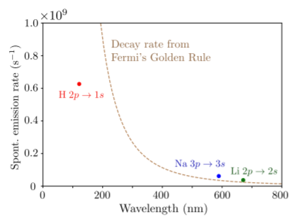
The figure below compares this prediction to experimentally-determined decay rates for the simplest excited states of hydrogen, lithium, and sodium atoms. The experimental data are derived from atomic emission line-widths, and correspond to the rate of spontaneous emission (also called the “Einstein \(A\) coefficient”) as the excited state decays to the ground state. For the Fermi’s Golden Rule curve, we simply approximated the transition dipole moment as \(|\mathbf{d}| \approx 10^{-10}\,\mathrm{m}\) (based on the fact that \(|\mathbf{d}|\) has units of length, and the length scale of an atomic orbital is about an angstrom); to be more precise, \(\mathbf{d}\) ought to be calculated using the actual orbital wavefunctions. Even with the crude approximations we have made, the predictions are within striking distance of the experimental values.