3.5: Intrinsic Quantities

Models can be dangerous, because they can tempt us to impute physical reality to features that are purely extrinsic, i.e., that are only present in that particular model. This is as opposed to intrinsic features, which are present in all models, and which are therefore logically implied by the axioms of the system itself. The existence of lunes is clearly an intrinsic feature of non-Euclidean geometries, because intersection of lines was defined before any model has even been proposed.

Example 4: Curvature in elliptic geometry

What about curvature? In the spherical model of elliptic geometry, the size of the sphere is an inverse measure of curvature. Is this a valid intrinsic quantity, or is it extrinsic? It seems suspect, because it is a feature of the model. If we try to define “size” as the radius R of the sphere, there is clearly reason for concern, because this seems to refer to the center of the sphere, but existence of a three-dimensional Euclidean space inside and outside the surface is clearly an extrinsic feature of the model. There is, however, a way in which a creature confined to the surface can determine R, by constructing geodesic and an affine parameter along that geodesic, and measuring the distance \(\lambda\) accumulated until the geodesic returns to the initial point. Since antipodal points are identified, \(\lambda\) equals half the circumference of the sphere, not its whole circumference, so R = \(\frac{\lambda}{\pi}\), by wholly intrinsic methods.

Example 5: Extrinsic curvature

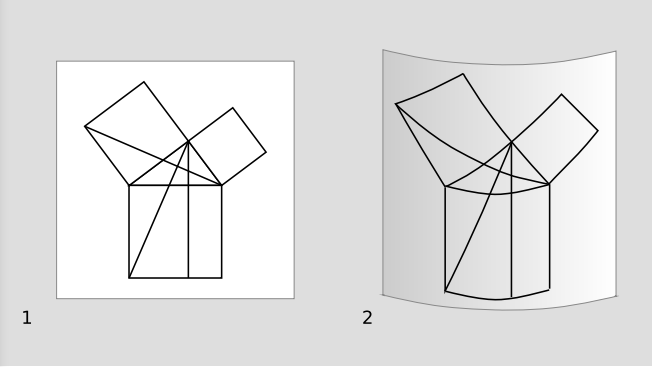
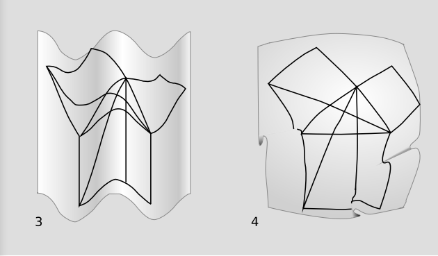
Euclid’s axioms E1-E5 refer to explicit constructions. If a two-dimensional being can physically verify them all as descriptions of the two-dimensional space she inhabits, then she knows that her space is Euclidean, and that propositions such as the Pythagorean theorem are physically valid in her universe. But the diagram in a/1 illustrating illustrating the proof of the Pythagorean theorem in Euclid’s Elements (proposition I.47) is equally valid if the page is rolled onto a cylinder, 2, or formed into a wavy corrugated shape, 3. These types of curvature, which can be achieved without tearing or crumpling the surface, are extrinsic rather than intrinsic. Of the curved surfaces in Figure 3.4.1, only the sphere, 4, has intrinsic curvature; the diagram can’t be plastered onto the sphere without folding or cutting and pasting.

Figure \(\PageIndex{1}\)

Exercise \(\PageIndex{1}\)

Self-check: How would the ideas of example 5 apply to a cone?

Example 5 shows that it can be difficult to sniff out bogus extrinsic features that seem intrinsic, and example 4 suggests the desirability of developing methods of calculation that never refer to any extrinsic quantities, so that we never have to worry whether a symbol like R staring up at us from a piece of paper is intrinsic. This is why it is unlikely to be helpful to a student of general relativity to pick up a book on differential geometry that was written without general relativity specifically in mind. Such books have a tendency to casually mix together intrinsic and extrinsic notation. For example, a vector cross product a × b refers to a vector poking out of the plane occupied by a and b, and the space outside the plane may be extrinsic; it is not obvious how to generalize this operation to the 3+1 dimensions of relativity (since the cross product is a three-dimensional beast), and even if it were, we could not be assured that it would have any intrinsically well defined meaning.

Coordinate Independence

To see how to proceed in creating a manifestly intrinsic notation, consider the two types of intrinsic observations that are available in general relativity:

• 1. We can tell whether events and world-lines are incident: whether or not two lines intersect, two events coincide, or an event lies on a certain line.

Incidence measurements, for example detection of gravitational lensing, are global, but they are the only global observations we can do.⁴ If we were limited entirely to incidence, spacetime would be described by the austere system of projective geometry, a geometry without parallels or measurement. In projective geometry, all propositions are essentially statements about combinatorics, e.g., that it is impossible to plant seven trees so that they form seven lines of three trees each.

Note

Einstein referred to incidence measurements as “determinations of spacetime coincidences.” For his presentation of this idea, see Appendix A.

But:

• 2. We can also do measurements in local Lorentz frames.

This gives us more power, but not as much as we might expect. Suppose we define a coordinate such as t or x. In Newtonian mechanics, these coordinates would form a predefined background, a preexisting stage for the actors. In relativity, on the other hand, consider a completely arbitrary change of coordinates of the form x → x' = f(x), where f is a smooth one-to-one function. For example, we could have x → x + px³ + q sin(rx) (with p and q chosen small enough so that the mapping is always one-to-one). Since the mapping is one-to-one, the new coordinate system preserves all the incidence relations. Since the mapping is smooth, the new coordinate system is still compatible with the existence of local Lorentz frames. The difference between the two coordinate systems is therefore entirely extrinsic, and we conclude that a manifestly intrinsic notation should avoid any explicit reference to a coordinate system. That is, if we write a calculation in which a symbol such as x appears, we need to make sure that nowhere in the notation is there any hidden assumption that x comes from any particular coordinate system. For example, the equation should still be valid if the generic symbol x is later taken to represent the distance r from some center of symmetry. This coordinate-independence property is also known as general covariance, and this type of smooth change of coordinates is also called a diffeomorphism.

Example 6:

As an exotic example of a change of coordinates, take a torus and label it with coordinates \(( \theta, \varphi)\), where \(\theta + 2 \pi\) is taken to be the same as \(\theta\), and similarly for \(\varphi\). Now subject it to the coordinate transformation T defined by \(\theta \rightarrow \theta + \varphi\), which is like opening the torus, twisting it by a full circle, and then joining the ends back together. T is known as the “Dehn twist,” and it is different from most of the coordinate transformations we do in relativity because it can’t be done smoothly, i.e., there is no continuous function f(x) on 0 ≤ x ≤ 1 such that every value of f is a smooth coordinate transformation, f(0) is the identity transformation, and f(1) = T.

Frames Moving at c?

A good application of these ideas is to the question of what the world would look like in a frame of reference moving at the speed of light. This question has a long and honorable history. As a young student, Einstein tried to imagine what an electromagnetic wave would look like from the point of view of a motorcyclist riding alongside it. We now know, thanks to Einstein himself, that it really doesn’t make sense to talk about such observers.

The most straightforward argument is based on the positivist idea that concepts only mean something if you can define how to measure them operationally. If we accept this philosophical stance (which is by no means compatible with every concept we ever discuss in physics), then we need to be able to physically realize this frame in terms of an observer and measuring devices. But we can’t. It would take an infinite amount of energy to accelerate Einstein and his motorcycle to the speed of light.

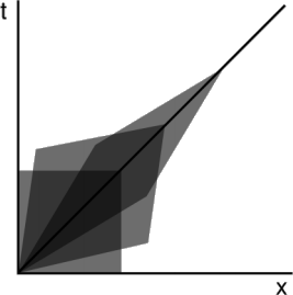
Since arguments from positivism can often kill off perfectly interesting and reasonable concepts, we might ask whether there are other reasons not to allow such frames. There are. Recall that we placed two technical conditions on coordinate transformations: they are supposed to be smooth and one-to-one. The smoothness condition is related to the inability to boost Einstein’s motorcycle into the speed-of-light frame by any continuous, classical process. (Relativity is a classical theory.) But independent of that, we have a problem with the one-to-one requirement. Figure 3.4.2 shows what happens if we do a series of Lorentz boosts to higher and higher velocities. It should be clear that if we could do a boost up to a velocity of c, we would have effected a coordinate transformation that was not one-to-one. Every point in the plane would be mapped onto a single lightlike line.

Figure \(\PageIndex{2}\) - A series of Lorentz boosts acts on a square.