8.7: Cosmological Solutions (Part 4)

The Radiation-dominated Solution

For the reasons discussed in example 14, the early universe was dominated by radiation. The solution of the Friedmann equations for this case is taken up in problem 11.

Local Effects of Expansion

In this section we discuss the predictions of general relativity concerning the effect of cosmological expansion on small, gravitationally bound systems such as the solar system or clusters of galaxies. The short answer is that in most realistic cosmologies (but not necessarily in “Big Rip” scenarios) the effect of expansion is not zero, but is many orders of magnitude too small to measure. Many readers will probably be willing to accept these assertions while skipping the following demonstrations.

To begin with, we observe that there are two qualitatively distinct types of effects that could exist. Suppose that a loaf of raisin bread is rising. Let’s say that the loaf’s scale factor a doubles by the time the yeast’s efforts are spent. By definition, this means that the raisins (galaxies, test particles) get farther apart by a factor of 2. We could imagine that in addition: (1) the strain of expansion could cause each raisin to puff up by, say, 1%, and to maintain this increased size over the entire course of expansion; or that (2) expansion could could cause each raisin to expand gradually, to 0.2% more than its original size, then 0.4% more than its original size, and so on, until, at the end of the process, each had grown beyond its original size by some amount such as 3.8%, which, while less than the 100% growth of the inter-raisin distances, was nevertheless nonzero. Astronomers refer to the second possibility as a “secular” trend. For example, simulations of solar systems often show that over billions of years, planets gradually migrate either inward or outward, under the influence of their gravitational interactions with other planets. As an example of an expansion without a secular trend, asteroids may experience a nonnegligible \(\frac{1}{r^{2}}\) force due to radiation pressure from the sun. The effect is exactly as if the sun’s mass or the gravitational constant had been slightly reduced. Kepler’s elliptical orbit law holds, the law of periods is slightly off, and the orbital radius shows zero trend over time.

If either type of effect exists, an observer in some local inertial frame will interpret it as a “force.” (The scare quotes are a reminder that general relativity doesn’t describe gravity as Newton-style linearly additive, instantaneous action at a distance.) Such a force, if it exists, cannot simply be proportional to the rate of expansion \(\frac{\dot{a}}{a}\). As a counterexample, the Milne universe is just flat spacetime described in silly coordinates, and it has \(\dot{a} \neq 0\).

It would make more sense for the force to depend on the second derivative of the scale factor. To justify this more precisely, imagine releasing two test particles, initially separated by some distance that is much less than the Hubble scale. They are initially at rest relative to the Hubble flow, and no locally gravitating bodies are present. As discussed in example 15, the acceleration of one test particle relative to the other is given by \((\frac{\ddot{a}}{a}\))r, where r is their relative displacement.

Thus if we are to observe any nonzero effects of expansion on a local system, they are not really effects of expansion at all, but effects of the acceleration of expansion. The factor \(\frac{\ddot{a}}{a}\) is on the order of the inverse square of the age of the universe, i.e., H²_o ∼ 10⁻³⁵ s⁻². The smallness of this factor is what makes the effect on a system such as the solar system so absurdly tiny.

Example 24: A human body

Let’s estimate the effect of cosmological expansion on the length L of your thigh bone. The body is made of atoms, and for the reasons given earlier, there can be no steady trend in the sizes of these atoms or the lengths of the chemical bonds between them. The bone experiences a stress due to cosmological expansion, but it is in equilibrium, and the strain will disappear if the gravitational stress is removed (e.g., if other gravitational stresses are superimposed on top of the cosmological one in order to cancel it). The anomalous acceleration between the ends of the bone is (\(\frac{\ddot{a}}{a}\))L, which is observed as an anomalous stress. Taking \(\frac{\ddot{a}}{a} \sim H^{2}_{o}\), the anomalous acceleration of one end of the bone relative to the other is ∼ LH². The corresponding compression or tension is ∼ mLH², where m is your body mass. The resulting strain is \(\epsilon\) ∼ \(\frac{mLH^{2}}{AE}\), where E is the Young’s modulus of bone (about 10¹⁰ Pa) and A is the bone’s cross-sectional area.

Putting in numbers, the result for the strain is about 10⁻⁴⁰, which is much too small to be measurable by any imaginable technique, and would in reality be swamped by other effects. Since the sign of a¨ is currently positive, this strain is tensile, not compressive. In the earlier, matter-dominated era of the universe, it would have been compressive.

There is no “secular trend,” i.e., your leg bone is not expanding over time. It’s in equilibrium, and is simply elongated imperceptibly compared to the length if would have had without the effect of cosmological expanson.

Example 25: strain on an atomic nucleus

The estimate in example 24 can also be applied to an atomic nucleus, which has a nuclear “Young’s modulus” on the order of 1 MeV/fm³ ∼ 10³² Pa. The result is a strain \(\epsilon\) ∼ 10⁻⁵² .

Example 26: a big rip

Known forms of matter are believed to have equations of state P = w\(\rho\) with w ≥ −1. The value for a vacuum-dominated universe would be w = −1. Cosmological observations²³ show that empirically the present-day universe behaves as if it is made out of stuff with w = −1.03 ± .16, and this leaves open the possibility of w < −1. In this case, the solution to the Friedmann equations gives a scale factor a(t) that blows up to infinity at some finite t. In such a scenario, known as a “Big Rip,” \((\frac{d}{dt})(\frac{\ddot{a}}{a})\) diverges, and any system, no matter how tightly bound, is ripped apart.²⁴

---

²³ Carnero et al., arxiv.org/abs/1104.5426

²⁴ Caldwell et al., arxiv.org/abs/astro-ph/0302506

Examples 24-26 show that except under hypothetical extreme cosmological conditions, there is no hope of detecting any effect of cosmological expansion on systems made of condensed matter. We need to look at much larger systems to see any effect, and such systems are held together by gravity. For concreteness, let’s keep talking about the earth-sun system. Not only is the anomalous force on the earth small, it is not guaranteed to produce any secular trend, which is what would be most likely to be detectable. The direction of the anomalous force on the earth is outward for an accelerating cosmological expansion, as we now know is the case for the present epoch. As an example in which no secular trend occurs, a vacuum-dominated cosmology gives a constant value for \(\frac{\ddot{a}}{a}\), so the outward force is constant. As with the effect of radiation pressure, the existence of this constant, outward force is very nearly equivalent to rescaling the sun’s gravitational force by a tiny amount, so the motion is still very nearly Keplerian, but with a slightly “wrong” constant of proportionality in Kepler’s law of periods. The rate of change \(\dot{r}\) in the radius of the circular orbit is therefore zero in this case.

But in most cosmologies \(\frac{\ddot{a}}{a}\) is not exactly constant, and the anomalous force on the earth varies. In a matter-dominated cosmology with \(\Lambda\) = 0, in its expanding phase, the force is inward but decreasing over time, so the orbit expands over time. What really matters then, is \((\frac{d}{dt})(\frac{\ddot{a}}{a})\). If we were free to pick any function for a(t), we could make up examples in which \(\dot{a}\) > 0 but \((\frac{d}{dt})(\frac{\ddot{a}}{a})\) < 0, so that the solar system would respond to cosmological expansion by shrinking!

The function a(t), however, has to satisfy the Friedmann equations, one of which is (in units with G ≠ 1)

\[\frac{\ddot{a}}{a} = G \Big[ \dfrac{1}{3} \Lambda - \frac{4 \pi}{3} (\rho + 3P) \Big] \ldotp \tag{8.2.18} \]

The present epoch of the universe seems to be well modeled by dark energy described by a constant \(\Lambda\) plus dust with P << \(\rho\). Differentiating both sides with respect to time gives

\[\dfrac{d}{dt} \left(\dfrac{\ddot{a}}{a}\right) \propto \dot{\rho}, \tag{8.2.19} \]

with a negative constant of proportionality. This ensures that the sign of the effect is always as expected from the naive Manichean image of binding forces struggling against cosmological expansion (or perhaps cooperating during the contracting phase of a Big Crunch cosmology).

One way of understanding why this reduces so nicely to a dependence on \(\dot{\rho}\) is the reasoning given in example 15, in which we found that the relative acceleration of two test particles A and B in a matter-dominated FRW cosmology could be calculated accurately by pretending that it was due to the presence of the dust in any given sphere S surrounding the two particles. We now let A be the sun, B the earth, and S a sphere centered on the sun whose radius equals the radius of the earth’s circular orbit. Due to cosmological expansion, the dust inside S thins out with time, reducing its density \(\rho\). Applying Newton’s laws to the orbit of the earth gives \(\omega^{2} r = \frac{GM}{r^{2}}\), and conservation of angular momentum results in \(\omega\)r² = const. A calculation gives $$\frac{r}{r_{o}} = \frac{M + (\frac{4 \pi}{3}) \rho_{o} r^{3}_{o}}{M + (\frac{4 \pi}{3}) \rho r^{3}} \tag{8.2.20} $$, which results in \(\frac{\dot{r}}{r_{o}} \approx −(\frac{4 \pi}{3})G \omega^{−2}_{o} \dot{\rho}\). Application of the Friedmann equations yields

\[\frac{\dot{r}}{r_{o}} = \omega^{-2}_{o} \left(\dfrac{d}{dt}\right) \left(\frac{\ddot{a}}{a}\right), \tag{8.2.21} \]

which is valid generally, not just for P = 0. The \(\omega^{−2}_{o}\) factor shows that the effect is smaller for more tightly bound systems.

We know that the universe in the present era has \((\frac{d}{dt})(\frac{\ddot{a}}{a})\) > 0 because \(\dot{\rho}\) < 0, and for purposes of an order-of-magnitude estimate we can take \((\frac{d}{dt})(\frac{\ddot{a}}{a}) \sim H^{3}_{o}\). Plugging in numbers for the earth-sun system, we find that since the age of the dinosaurs, the radius of the earth’s orbit has grown by less than the diameter of an atomic nucleus.²⁵

Note

The picturesque image comes from Cooperstock et al., http://arxiv.org/abs/astro-ph/9803097v1, who give a different calculation leading to a result for \(\dot{r}\) exactly equivalent to the one derived here.

Observations

Historically, it was believed that the cosmological constant was zero, that nearly all matter in the universe was in the form of atoms, and that there was therefore only one interesting cosmological parameter to measure, which was the average density of matter. This density was very difficult to determine, even to within an order of magnitude, because most of the matter in the universe probably doesn’t emit light, making it difficult to detect. Astronomical distance scales were also very poorly calibrated against absolute units such as the SI. Starting around 1995, however, a new set of techniques led to an era of high-precision cosmology.

Spatial Curvature from CMB Fluctuations

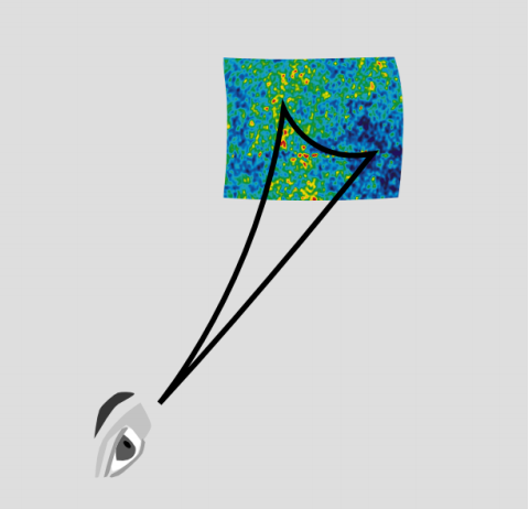
A strong constraint on the models comes from accurate measurements of the cosmic microwave background, especially by the 1989-1993 COBE probe, and its 2001-2009 successor, the Wilkinson Microwave Anisotropy Probe, positioned at the L2 Lagrange point of the earth-sun system, beyond the Earth on the line connecting sun and earth.²⁶ The temperature of the cosmic microwave background radiation is not the same in all directions, and it can be measured at different angles. In a universe with negative spatial curvature, the sum of the interior angles of a triangle is less than the Euclidean value of 180 degrees. Therefore if we observe a variation in the CMB over some angle, the distance between two points on the surface of last scattering is actually greater than would have been inferred from Euclidean geometry. The distance scale of such variations is limited by the speed of sound in the early universe, so one can work backward and infer the universe’s spatial curvature based on the angular scale of the anisotropies. The measurements of spatial curvature are usually stated in terms of the parameter \(\Omega\), defined as the total average density of all source terms in the Einstein field equations, divided by the critical density that results in a flat universe. \(\Omega\)includes contributions from matter, \(\Omega_{M}\), the cosmological constant, \(\Omega_{\Lambda}\), and radiation (negligible in the present-day universe). The results from WMAP, combined with other data from other methods, gives \(\Omega\) = 1.005 ± .006. In other words, the universe is very nearly spatially flat.

Figure \(\PageIndex{6}\) - The angular scale of fluctuations in the cosmic microwave background can be used to infer the curvature of the universe.

Accelerating Expansion from Supernova Data

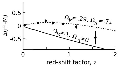
The supernova data described in section 8.2 complement the CMB data because they are mainly sensitive to the difference \(\Omega_{\Lambda} − \Omega_{M}\), rather than their sum \(\Omega = \Omega_{\Lambda} + \Omega_{M}\). This is because these data measure the acceleration or deceleration of the universe’s expansion. Matter produces deceleration, while the cosmological constant gives acceleration. Figure 8.2.7 shows some recent supernova data.²⁷ The horizontal axis gives the redshift factor z = \(\frac{\lambda' − \lambda}{\lambda}\), where \(\lambda'\) is the wavelength observed on earth and \(\lambda\) the wavelength originally emitted. It measures how fast the supernova’s galaxy is receding from us. The vertical axis is \(\Delta\)(m−M) = (m−M)−(m−M)_empty, where m is the apparent magnitude, M is the absolute magnitude, and (m − M)_empty is the value expected in a model of an empty universe, with \(\Omega\) = 0. The difference m−M is a measure of distance, so essentially this is a graph of distance versus recessional velocity, of the same general type used by Hubble in his original discovery of the expansion of the universe. Subtracting (m−M)_empty on the vertical axis makes it easier to see small differences. Since the WMAP data require \(\Omega\) = 1, we need to fit the supernova data with values of \(\Omega_{M}\) and \(\Omega_{\Lambda}\) that add up to one. Attempting to do so with \(\Omega_{M}\) = 1 and \(\Omega_{\Lambda}\) = 0 is clearly inconsistent with the data, so we can conclude that the cosmological constant is definitely positive.

Figure \(\PageIndex{7}\) - A Hubble plot for distant supernovae. Each data point represents an average over several different supernovae with nearly the same z.

Density of Matter from Baryonic Acoustic Oscillations

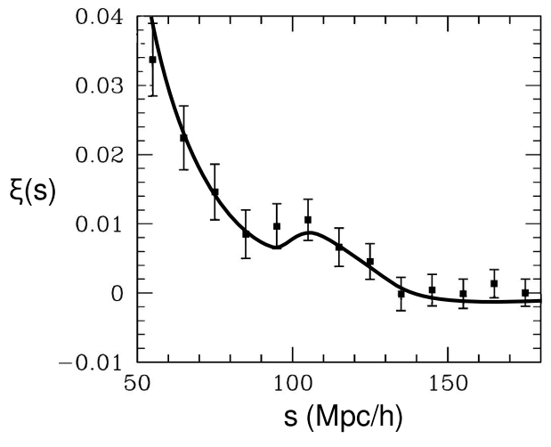
Efforts such as the Sloan Digital Sky Survey have made threedimensional maps of the density of luminous matter in the universe.²⁸ The distribution is clumpy. Measuring the average correlation \(\xi\) between the density at points separated by some distance s (measured in the comoving frame), one would expect that the function \(\xi\)(s) would be largest when s was small and would simply taper off with increasing s. By analogy, we don’t usually find a Manhattan-style landscape of skyscrapers side by side with an uninhabited mountainous wilderness. On the other hand, imagine constructing such a correlation function for houses in a subdivision in which the roads do not form any regular grid, but zoning regulations prohibit construction of houses on lots of less than a certain size. In this situation, there would be zero probability of finding houses separated by very small distances, and \(\xi\)(s) would exhibit a peak at some larger scale set by the legal code. The actual results of the sky surveys do show such a peak, which is due to well known physics referred to as baryon acoustic oscillations (BAO).²⁹ In the early universe, any region of overdensity would tend to create a radiating sound wave like the bang of a firecracker. Such waves propagated at a known speed (about half the speed of light) for a known time (about 400,000 years, until matter became deionized and transparent to radiation, making it immune to the photon pressure that drove the oscillations). This leads to a known distance s, which forms a standard ruler at which the peak in \(\xi\)(s) occurs. In cosmological models, these results strongly constrain \(\Omega_{M}\), while being relatively insensitive to \(\Omega_{\Lambda}\), and they are therefore complementary to both the supernova data and the CMB results.

Figure \(\PageIndex{8}\) - The acoustic peak in the BAO correlation function. Redrawn from Eisenstein, New Astronomy Reviews. 49 (2005) 360, as reproduced in Bassett and Hlozek, 2009, arxiv.org/abs/0910.5224.

Conclusions about Cosmology

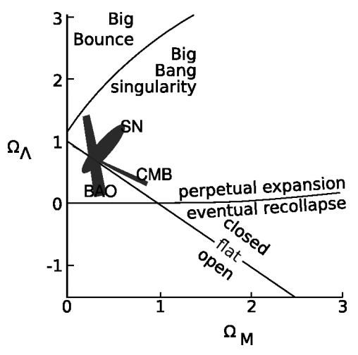
Figure 8.2.9 summarizes what we can conclude about our universe, parametrized in terms of a model with both \(\Omega_{M}\) and \(\Omega_{\Lambda}\) nonzero.³⁰ We can tell that it originated in a Big Bang singularity, that it will go on expanding forever, and that it is very nearly flat. Note that in a cosmology with nonzero values for both \(\Omega_{M}\) and \(\Omega_{\Lambda}\), there is no strict linkage between the spatial curvature and the question of recollapse, as there is in a model with only matter and no cosmological constant; therefore even though we know that the universe will not recollapse, we do not know whether its spatial curvature is slightly positive (closed) or negative (open).

Figure \(\PageIndex{9}\) - The cosmological parameters of our universe, after Perlmutter, 1998, arxiv.org/abs/astro-ph/9812133 and Kowalski, 2008, arxiv.org/abs/0804.4142. The three shaded regions represent the 95% confidence regions for the three types of observations.

Consistency Checks

Astrophysical considerations provide further constraints and consistency checks. In the era before the advent of high-precision cosmology, estimates of the age of the universe ranged from 10 billion to 20 billion years, and the low end was inconsistent with the age of the oldest globular clusters. This was believed to be a problem either for observational cosmology or for the astrophysical models used to estimate the age of the clusters: “You can’t be older than your ma.” Current data have shown that the low estimates of the age were incorrect, so consistency is restored.

That only a small fraction of the universe’s matter was luminous had been suspected by astronomers such as Zwicky as early as 1933, based on the inability to reconcile the observed kinematics with Newton’s laws if all matter was assumed to be luminous.

Dark Matter

Another constraint comes from models of nucleosynthesis during the era shortly after the Big Bang (before the formation of the first stars). The observed relative abundances of hydrogen, helium, and deuterium cannot be reconciled with the density of “dust” (i.e., nonrelativistic matter) inferred from the observational data. If the inferred mass density were entirely due to normal “baryonic” matter (i.e., matter whose mass consisted mostly of protons and neutrons), then nuclear reactions in the dense early universe should have proceeded relatively efficiently, leading to a much higher ratio of helium to hydrogen, and a much lower abundance of deuterium. The conclusion is that most of the matter in the universe must be made of an unknown type of exotic non-baryonic matter, known generically as “dark matter.”

The existence of nonbaryonic matter is also required in order to reconcile the observed density of galaxies with the observed strength of the CMB fluctuations, and in merging galaxy clusters it has been observed that the gravitational potential is offset from the radiating plasma. A 2012 review paper on dark matter is Roos, arxiv.org/abs/1208.3662.

A number of experiments are under way to detect dark matter directly. As of 2013, the most sensitive experiment has given null results: arxiv.org/abs/1310.8214.

At one time it was widely expected that dark matter would consist of the lightest supersymmetric particle, which might for example be the neutralino. However, results from the LHC seem to make it unlikely that our universe exhibits supersymmetry, assuming that the energy scale is the electroweak scale, which is the only scale that has strong motivation. It now appears more likely that dark matter consists of some other particle such as sterile neutrinos or axions. Even with the inclusion of dark matter, there is a problem with the abundance of lithium-7 relative to hydrogen, which models greatly overpredict.³¹

References

²⁶ Komatsu et al., 2010, arxiv.org/abs/1001.4538

²⁷ Riess et al., 2007, arxiv.org/abs/astro-ph/0611572. A larger data set is analyzed in Kowalski et al., 2008, arxiv.org/abs/0804.4142.

²⁸ Sanchez et al., 2012, arxiv.org/abs/1203.6616

²⁹ Bassett and Hlozek, 2009, arxiv.org/abs/0910.5224

³⁰ See Carroll, “The Cosmological Constant,” http://www.livingreviews.org/lrr-2001-1 for a full mathematical treatment of such models.

³¹ arxiv.org/abs/0808.2818, arxiv.org/abs/1107.1117