1.1: Introduction - Statistical physics and thermodynamics

Statistical physics (alternatively called “statistical mechanics”) and thermodynamics are two different but related approaches to the same goal: an approximate description of the “internal”² properties of large physical systems, notably those consisting of \(N >> 1\) identical particles – or other components. The traditional example of such a system is a human-scale portion of gas, with the number \(N\) of atoms/molecules³ of the order of the Avogadro number \(N_A \sim 10^{23}\) (see Sec. 4 below).

The motivation for the statistical approach to such systems is straightforward: even if the laws governing the dynamics of each particle and their interactions were exactly known, and we had infinite computing resources at our disposal, calculating the exact evolution of the system in time would be impossible, at least because it is completely impracticable to measure the exact initial state of each component – in the classical case, the initial position and velocity of each particle. The situation is further exacerbated by the phenomena of chaos and turbulence,⁴ and the quantum-mechanical uncertainty, which do not allow the exact calculation of final positions and velocities of the component particles even if their initial state is known with the best possible precision. As a result, in most situations, only statistical predictions about the behavior of such systems may be made, with the probability theory becoming a major tool of the mathematical arsenal.

However, the statistical approach is not as bad as it may look. Indeed, it is almost self-evident that any measurable macroscopic variable characterizing a stationary system of \(N >> 1\) particles as a whole (think, e.g., about the stationary pressure \(P\) of the gas contained in a fixed volume \(V\)) is almost constant in time. Indeed, as we will see below, besides certain exotic exceptions, the relative magnitude of fluctuations – either in time, or among many macroscopically similar systems – of such a variable is of the order of \(1/N^{1/2}\), and for \(N \sim N_A\) is extremely small. As a result, the average values of appropriate macroscopic variables may characterize the state of the system quite well – satisfactory for nearly all practical purposes. The calculation of relations between such average values is the only task of thermodynamics and the main task of statistical physics. (Fluctuations may be important, but due to their smallness, in most cases their analysis may be based on perturbative approaches – see Chapter 5.)

Now let us have a fast look at the typical macroscopic variables the statistical physics and thermodynamics should operate with. Since I have already mentioned pressure \(P\) and volume \(V\), let me start with this famous pair of variables. First of all, note that volume is an extensive variable, i.e. a variable whose value for a system consisting of several non-interacting parts is the sum of those of its parts. On the other hand, pressure is an example of an intensive variable whose value is the same for different parts of a system – if they are in equilibrium. To understand why \(P\) and \(V\) form a natural pair of variables, let us consider the classical playground of thermodynamics, a portion of a gas contained in a cylinder, closed with a movable piston of area \(A\) (Figure \(\PageIndex{1}\)).

Figure \(\PageIndex{1}\): Compressing gas.

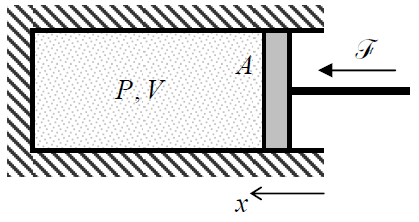
Neglecting the friction between the walls and the piston, and assuming that it is being moved so slowly that the pressure \(P\) is virtually the same for all parts of the volume at any instant, the elementary work of the external force \(\mathscr{F} = PA\), compressing the gas, at a small piston displacement \(dx = –dV/A\), is

Work on a gas:

\[\boxed{d\mathscr{W} = \mathscr{F}dx = \left(\frac{\mathscr{F}}{A}\right) (Adx) = -PdV.} \label{1}\]

Of course, the last expression is more general than the model shown in Figure \(\PageIndex{1}\), and does not depend on the particular shape of the system’s surface.⁵ (Note that in the notation of Equation (\ref{1}), which will be used through the course, the elementary work done by the gas on the external system equals \(–d\mathscr{W}\).)

From the point of analytical mechanics,⁶ \(V\) and \((–P)\) is just one of many possible canonical pairs of generalized coordinates \(q_j\) and generalized forces \(\mathscr{F}_j\), whose products \(d\mathscr{W}_j = \mathscr{F}_jdq_j\) give independent contributions to the total work of the environment on the system under analysis. For example, the reader familiar with the basics of electrostatics knows that if the spatial distribution \( \pmb{\mathscr{E}}\mathbf{(r)}\) of an external electric field does not depend on the electric polarization \(\pmb{\mathscr{P}} \mathbf{(r)}\) of a dielectric medium placed into the field, its elementary work on the medium is

\[d \mathscr{W}=\int \pmb{\mathscr{E}}(\mathbf{r}) \cdot d \pmb{\mathscr{P}}(\mathbf{r}) d^{3} r \equiv \int \sum_{j=1}^{3} \mathscr{E}_{j}(\mathbf{r}) d \mathscr{P}_{j}(\mathbf{r}) d^{3} r . \label{2a}\]

\[d \mathscr{W}=\sum_{k} d \mathscr{W}_{k}, \quad \text{ with } d \mathscr{W}_{k}=\pmb{\mathscr{E}} \left(\mathbf{r}_{k}\right) \cdot d \pmb{\mathcal{p}}_{k} .\label{2b}\]

\[\begin{align} d \mathscr{W}=\mu_{0} \int \pmb{\mathscr{H}}(\mathbf{r}) \cdot d \pmb{\mathscr{M}}(\mathbf{r}) d^{3} r \equiv \mu_{0} \int \sum_{j=1}^{3} \mathscr{H}_{j}(\mathbf{r}) d \mathscr{M}_{j}(\mathbf{r}) d^{3} r, \label{3a} \\ d \mathscr{W}=\sum_{k} d \mathscr{W}_{k}, \quad \text{ with } d \mathscr{W}_{k}=\mu_{0} \pmb{\mathscr{H}} \left(\mathbf{r}_{k}\right) \cdot d \pmb{\mathcal{m}}_{k} \label{3b}. \end{align} \]

where \(\pmb{\mathscr{M}}\) and \(\pmb{\mathcal{m}}\) are the vectors of, respectively, the medium’s magnetization and the magnetic moment of a single dipole. Formulas (\ref{2a} - \ref{2b}) and (\ref{3a} - \ref{3b}) show that the roles of generalized coordinates may be played by Cartesian components of the vectors \(\pmb{\mathscr{P}}\) (or \(\pmb{\mathcal{p}}\)) and \(\pmb{\mathscr{M}}\) (or \(\pmb{\mathcal{m}}\)), with the components of the electric and magnetic fields playing the roles of the corresponding generalized forces. This list may be extended to other interactions (such as gravitation, surface tension in fluids, etc.). Following tradition, I will use the \(\{–P, V \}\) pair in almost all the formulas below, but the reader should remember that they all are valid for any other pair \(\{\mathscr{F}_j, q_j\}\).⁹

Again, the specific relations between the variables of each pair listed above may depend on the statistical properties of the system under analysis, but their definitions are not based on statistics. The situation is very different for a very specific pair of variables, temperature \(T\) and entropy \(S\), although these “sister variables” participate in many formulas of thermodynamics exactly as if they were just one more canonical pair \(\{\mathscr{F}_j, q_j\}\). However, the very existence of these two notions is due to statistics. Namely, temperature \(T\) is an intensive variable that characterizes the degree of thermal “agitation” of the system’s components. On the contrary, the entropy \(S\) is an extensive variable that in most cases evades immediate perception by human senses; it is a qualitative measure of the disorder of the system, i.e. the degree of our ignorance about its exact microscopic state.¹⁰

The reason for the appearance of the \(\{T, S\}\) pair of variables in formulas of thermodynamics and statistical mechanics is that the statistical approach to large systems of particles brings some qualitatively new results, most notably the notion of the irreversible time evolution of collective (macroscopic) variables describing the system. On one hand, the irreversibility looks absolutely natural in such phenomena as the diffusion of an ink drop in a glass of water. In the beginning, the ink molecules are located in a certain small part of the system’s volume, i.e. to some extent ordered, while at the late stages of diffusion, the position of each molecule in the glass is essentially random. However, as a second thought, the irreversibility is rather surprising, taking into account that the laws governing the motion of the system’s components are time-reversible – such as the Newton laws or the basic laws of quantum mechanics.¹¹ Indeed, if at a late stage of the diffusion process, we reversed the velocities of all molecules exactly and simultaneously, the ink molecules would again gather (for a moment) into the original spot.¹² The problem is that getting the information necessary for the exact velocity reversal is not practicable. This example shows a deep connection between statistical mechanics and information theory.

A qualitative discussion of the reversibility-irreversibility dilemma requires a strict definition of the basic notion of statistical mechanics (and indeed of the probability theory), the statistical ensemble, and I would like to postpone it until the beginning of Chapter 2. In particular, in that chapter, we will see that the basic law of irreversible behavior is an increase of the entropy \(S\) in any closed system. Thus, the statistical mechanics, without defying the “microscopic” laws governing the evolution of system’s components, introduces on top of them some new “macroscopic” laws, intrinsically related to the evolution of information, i.e. the degree of our knowledge of the microscopic state of the system.

To conclude this brief discussion of variables, let me mention that as in all fields of physics, a very special role in statistical mechanics is played by the energy \(E\). To emphasize the commitment to disregard the motion of the system as a whole in this subfield of physics, the \(E\) considered in thermodynamics it is frequently called the internal energy, though just for brevity, I will skip this adjective in most cases. The simplest example of such \(E\) is the sum of kinetic energies of molecules in a dilute gas at their thermal motion, but in general, the internal energy also includes not only the individual energies of the system’s components but also their interactions with each other. Besides a few “pathological” cases of very-long-range interactions, these interactions may be treated as local; in this case the internal energy is proportional to \(N\), i.e. is an extensive variable. As will be shown below, other extensive variables with the dimension of energy are often very useful as well, including the (Helmholtz) free energy \(F\), the Gibbs energy \(G\), the enthalpy \(H\), and the grand potential \(\Omega\). (The collective name for such variables is thermodynamic potentials.)

Now, we are ready for a brief discussion of the relationship between statistical physics and thermodynamics. While the task of statistical physics is to calculate the macroscopic variables discussed above¹³ for various microscopic models of the system, the main role of thermodynamics is to derive some general relations between the average values of the macroscopic variables (also called thermodynamic variables) that do not depend on specific models. Surprisingly, it is possible to accomplish such a feat using just a few either evident or very plausible general assumptions (sometimes called the laws of thermodynamics), which find their proof in statistical physics.¹⁴ Such general relations allow for a substantial reduction of the number of calculations we have to do in statistical physics: in most cases, it is sufficient to calculate from the statistics just one or two variables, and then use general thermodynamic relations to get all other properties of interest. Thus the thermodynamics, sometimes snubbed as a phenomenology, deserves every respect not only as a useful theoretical tool but also as a discipline more general than any particular statistical model. This is why the balance of this chapter is devoted to a brief review of thermodynamics.