
1.5: Systems with a variable number of particles


- Last updated
- Sep 20, 2022
- Save as PDF

( \newcommand{\kernel}{\mathrm{null}\,}\)
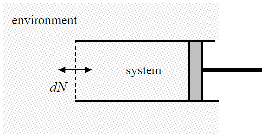
Now we have to consider one more important case: when the number N of particles in a system is not rigidly fixed, but may change as a result of a thermodynamic process. A typical example of such a system is a gas sample separated from the environment by a penetrable partition – see Figure 1.5.1.37
Let us analyze this situation for the simplest case when all the particles are similar. (In Sec. 4.1, this analysis will be extended to systems with particles of several sorts). In this case, we may consider N as an independent thermodynamic variable whose variation may change the energy E of the system, so that (for a slow, reversible process) Equation (1.3.4) should be now generalized as
dE=TdS−PdV+μdN,
where μ is a new function of state, called the chemical potential.38 Keeping the definitions of other thermodynamic potentials, given by Eqs. (1.4.4), (1.4.10), and (1.4.14), intact, we see that the expressions for their differentials should be generalized as
dH=TdS+VdP+μdN,dF=−SdT−PdV+μdN,,dG=−SdT+VdP+μdN
μ=(∂E∂N)S,V=(∂H∂N)S,P=(∂F∂N)T,V=(∂G∂N)T,P.
Despite the formal similarity of all Eqs. (???), one of them is more consequential than the others. Indeed, the Gibbs energy G is the only thermodynamic potential that is a function of two intensive parameters, T and P. However, as all thermodynamic potentials, G has to be extensive, so that in a system of similar particles it has to be proportional to N:
G=Ng,
where g is some function of T and P. Plugging this expression into the last of Eqs. (???), we see that μ equals exactly this function, so that
μ as Gibbs energy:
μ=GN,
i.e. the chemical potential is just the Gibbs energy per particle.
In order to demonstrate how vital the notion of chemical potential may be, let us consider the situation (parallel to that shown in Figure 1.2.1) when a system consists of two parts, with equal pressure and temperature, that can exchange particles at a relatively slow rate (much slower than the speed of the internal relaxation of each part). Then we can write two equations similar to Eqs. (1.2.2):
N=N1+N2,G=G1+G2
where N= const, and Equation (???) may be used to describe each component of G:
G=μ1N1+μ2N2
Plugging the N2 expressed from the first of Eqs. (???), N_2 = N – N_1, into Equation (\ref{58}), we see that
\frac{dG}{dN_1} = \mu_1 − \mu_2, \label{59}
so that the minimum of G is achieved at \mu_1 = \mu_2. Hence, in the conditions of fixed temperature and pressure, i.e. when G is the appropriate thermodynamic potential, the chemical potentials of the system parts should be equal – the so-called chemical equilibrium.
Finally, later in the course, we will also run into several cases when the volume V of a system, its temperature T, and the chemical potential \mu are all fixed. (The last condition may be readily implemented by allowing the system of our interest to exchange particles with an environment so large that its \mu stays constant.) The thermodynamic potential appropriate for this case may be obtained by subtraction of the product \mu N from the free energy F, resulting in the so-called grand thermodynamic (or “Landau”) potential:
\boxed{ \Omega \equiv F - \mu N = F - \frac{G}{N} N \equiv F - G = -PV. } \label{60}
Indeed, for a reversible process, the full differential of this potential is
Grand potential: differential
\boxed{ d\Omega = dF − d(\mu N) = (−SdT − PdV + \mu dN) − (\mu dN + Nd\mu ) = −SdT − PdV − Nd\mu , } \label{61}
so that if \Omega has been calculated as a function of T, V, and \mu , other thermodynamic variables may be found as
S = -\left( \frac{ \partial \Omega}{\partial T} \right)_{V, \mu}, \quad P = -\left( \frac{ \partial \Omega}{\partial V} \right)_{T, \mu}, \quad N = -\left( \frac{ \partial \Omega}{\partial \mu } \right)_{T, V}. \label{62}
Now acting exactly as we have done for other potentials, it is straightforward to prove that an irreversible process with fixed T, V, and \mu , provides d\Omega /dt \leq 0, so that system’s equilibrium indeed corresponds to the minimum of the grand potential \Omega . We will repeatedly use this fact in this course.