
1.6: Thermal machines


- Last updated
- Sep 20, 2022
- Save as PDF

( \newcommand{\kernel}{\mathrm{null}\,}\)
In order to complete this brief review of thermodynamics, I cannot completely pass the topic of thermal machines – not because it will be used much in this course, but mostly because of its practical and historic significance.40 Figure 1.6.1a shows the generic scheme of a thermal machine that may perform mechanical work on its environment (in our notation, equal to −W) during each cycle of the expansion/compression of some “working gas”, by transferring different amounts of heat from a high temperature heat bath (QH) and to the low-temperature bath (QL).
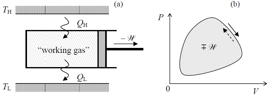
One relation between the three amounts QH, QL, and W is immediately given by the energy conservation (i.e. by the 1st law of thermodynamics):
QH−QL=−W.
From Equation (1.1.1), the mechanical work during the cycle may be calculated as
−W=∮PdV,
and hence represented by the area circumvented by the state-representing point on the [P,V] plane – see Figure 1.6.1b. Note that the sign of this circular integral depends on the direction of the point’s rotation; in particular, the work (–W) done by the working gas is positive at its clockwise rotation (pertinent to heat engines) and negative in the opposite case (implemented in refrigerators and heat pumps – see below). Evidently, the work depends on the exact form of the cycle, which in turn may depend not only on TH and TL, but also on the working gas’ properties.
An exception from this rule is the famous Carnot cycle, consisting of two isothermal and two adiabatic processes (all reversible!). In its heat engine’s form, the cycle may start, for example, from an isothermic expansion of the working gas in contact with the hot bath (i.e. at T=TH). It is followed by its additional adiabatic expansion (with the gas being disconnected from both heat baths) until its temperature drops to TL. Then an isothermal compression of the gas is performed in its contact with the cold bath (at T=TL), followed by its additional adiabatic compression to raise T to TH again, after which the cycle is repeated again and again. Note that during this cycle the working gas is never in contact with both heat baths simultaneously, thus avoiding the irreversible heat transfer between them. The cycle’s shape on the [V,P] plane (Figure 1.6.2a) depends on the exact properties of the working gas and may be rather complicated. However, since the system’s entropy is constant at any adiabatic process, the Carnot cycle’s shape on the [S,T] plane is always rectangular – see Figure 1.6.2b.
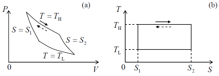
Since during each isotherm, the working gas is brought into thermal contact only with the corresponding heat bath, i.e. its temperature is constant, the relation (1.3.6), dQ=TdS, may be immediately integrated to yield
QH=TH(S2−S1),QL=TL(S2−S1).
Hence the ratio of these two heat flows is completely determined by their temperature ratio:
QHQL=THTL,
η≡|W|QH=QH−QLQH≡1−QLQH≤1.
Carnot cycle's efficiency:
ηCarnot−1−TLTH,
which shows that at a given TL (that is typically the ambient temperature ∼300 K), the efficiency may be increased, ultimately to 1, by raising the temperature TH of the heat source.42
On the other hand, if the cycle is reversed (see the dashed arrows in Figs. 1.6.1 and 1.6.2), the same thermal machine may serve as a refrigerator, providing heat removal from the low-temperature bath (QL<0) at the cost of consuming external mechanical work: W>0. This reversal does not affect the basic relation (???), which now may be used to calculate the relevant figure-of-merit, called the cooling coefficient of performance (COPcooling):
COPcooling≡|QL|W=QLQH−QL.
Notice that this coefficient may be above unity; in particular, for the Carnot cycle we may use Equation (???) (which is also unaffected by the cycle reversal) to get
(COPcooling)Carnot=TLTH−TL,
so that this value is larger than 1 at TH<2TL, and even may be much larger than that when the temperature difference (TH–TL) sustained by the refrigerator, tends to zero. For example, in a typical air-conditioning system, this difference is of the order of 10 K, while TL∼300 K, so that (TH–TL)∼TL/30, i.e. the Carnot value of COPcooling is as high as ∼30. (In the state-of-the-art commercial HVAC systems it is within the range of 3 to 4.) This is why the term “cooling efficiency”, used in some textbooks instead of (COP)cooling, may be misleading.
Since in the reversed cycle QH=–W+QL<0, i.e. the system provides heat flow into the high temperature heat bath, it may be used as a heat pump for heating purposes. The figure-of-merit appropriate for this application is different from Equation (???):
COPheating≡|QH|W=QHQH−QL,
so that for the Carnot cycle, using Equation (???) again, we get
(COPheating)Carnot=THTH−TL.
Note that this COP is always larger than 1, meaning that the Carnot heat pump is always more efficient than the direct conversion of work into heat (when QH=–W, so that COPheating = 1), though practical electricity-driven heat pumps are substantially more complex, and hence more expensive than simple electric heaters. Such heat pumps, with the typical COPheating values around 4 in summer and 2 in winter, are frequently used for heating large buildings.
Finally, note that according to Equation (???), the COPcooling of the Carnot cycle tends to zero at TL→0, making it impossible to reach the absolute zero of temperature, and hence illustrating the meaningful (Nernst’s) formulation of the 3rd law of thermodynamics, cited in Sec. 3. Indeed, let us prescribe a finite but very large heat capacity C(T) to the low-temperature bath, and use the definition of this variable to write the following expression for the relatively small change of its temperature as a result of dn similar refrigeration cycles:
C(TL)dTL=QLdn.
Together with Equation (???), this relation yields
C(TL)dTLTL=−|QH|THdn.
If TL→0, so that TH>>TL and |QH|≈–W= const, the right-hand side of this equation does not depend on TL, so that if we integrate it over many (n>>1) cycles, getting the following simple relation between the initial and final values of TL:
∫TfinTiniC(T)dTT=−|QH|THn.
For example, if C(T) is a constant, Equation (???) yields an exponential law,
Tfin=Tiniexp{−|QH|CTHn},
with the absolute zero of temperature not reached as any finite n. Even for an arbitrary function C(T) that does not vanish at T→0, Equation (???) proves the Nernst theorem, because dn diverges at TL→0. 45