
1.4: Thermodynamic potentials


( \newcommand{\kernel}{\mathrm{null}\,}\)
Since for a fixed volume, dW=–PdV=0, and Equation (1.3.5) yields dQ=dE, we may rewrite Equation (1.3.9) in another convenient form
CV−(∂E∂T)V.
so that to calculate CV from a certain statistical-physics model, we only need to calculate E as a function of temperature and volume. If we want to obtain a similarly convenient expression for CP, the best way is to introduce a new notion of so-called thermodynamic potentials – whose introduction and effective use is perhaps one of the most impressive techniques of thermodynamics. For that, let us combine Eqs. (1.1.1) and (1.3.5) to write the 1st law of thermodynamics in its most common form
dQ=dE+PdV
At an isobaric process (Figure 1.3.2), i.e. at P= const, this expression is reduced to
(dQ)P=dEP+d(PV)P=d(E+PV)P
H≡E+PV
called enthalpy (or, sometimes, the “heat function” or the “heat contents”),27 we may rewrite Equation (1.3.10) as
CP=(∂H∂T)P.
Comparing Eqs. (???) and (???) we see that for the heat capacity, the enthalpy H plays the same role at fixed pressure as the internal energy E plays at fixed volume.
Now let us explore properties of the enthalpy at an arbitrary reversible process, i.e. lifting the restriction P= const, but keeping the definition (???). Differentiating this equality, we get
dH=dE+PdV+VdP.
Plugging into this relation Equation (1.3.4) for dE, we see that the terms ±PdV cancel, yielding a very simple expression
Enthalpy: differential
dH=TdS+VdP,
whose right-hand side differs from Equation (1.3.4) only by the swap of P and V in the second term, with the simultaneous change of its sign. Formula (???) shows that if H has been found (say, experimentally measured or calculated for a certain microscopic model) as a function of the entropy S and the pressure P of a system, we can calculate its temperature T and volume V by simple partial differentiation:
T=(∂H∂S)P,V=(∂H∂P)S.
The comparison of the first of these relations with Equation (1.2.6) shows that not only for the heat capacity but for temperature as well, enthalpy plays the same role at fixed pressure, as played by internal energy at fixed volume.
This success immediately raises the question of whether we could develop this idea further on, by defining other useful thermodynamic potentials – the variables with the dimensionality of energy that would have similar properties – first of all, a potential that would enable a similar swap of T and S in its full differential, in comparison with Equation (???). We already know that an adiabatic process is the reversible process with fixed entropy, inviting analysis of a reversible process with fixed temperature. Such an isothermal process may be implemented, for example, by placing the system under consideration into thermal contact with a much larger system (called either the heat bath, or “heat reservoir”, or “thermostat”) that remains in thermodynamic equilibrium at all times – see Figure 1.4.1.
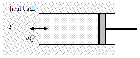
Due to its very large size, the heat bath temperature T does not depend on what is being done with our system, and if the change is being done sufficiently slowly (i.e. reversibly), that this temperature is also the temperature of our system – see Equation (1.2.5) and its discussion. Let us calculate the elementary mechanical work dW (1.1.1) at such a reversible isothermal process. According to the general Equation (1.3.5), dW=dE–dQ. Plugging dQ from Equation (1.3.6) into this equality, for T= const we get
(dW)T=dE−TdS=d(E−TS)≡dF,
where the following combination,
F≡E−TS,
is called the free energy (or the “Helmholtz free energy”, or just the “Helmholtz energy”28). Just as we have done for the enthalpy, let us establish properties of this new thermodynamic potential for an arbitrarily small, reversible (now not necessarily isothermal!) variation of variables, while keeping the definition (???). Differentiating this relation and then using Equation (1.3.4), we get
Free energy: differential
dF=−SdT−PdV.
Thus, if we know the function F(T,V), we can calculate S and P by simple differentiation:
S=−(∂F∂T)V,P=−(∂F∂V)T.
E=E(S,V);H=H(S,P);F=F(T,V).
In this list of pairs of four arguments, only one pair is missing: {T,P}. The thermodynamic function of this pair, which gives the two remaining variables (S and V) by simple differentiation, is called the Gibbs energy (or sometimes the “Gibbs free energy”): G=G(T,P). The way to define it in a symmetric way is evident from the so-called circular diagram shown in Figure 1.4.2.
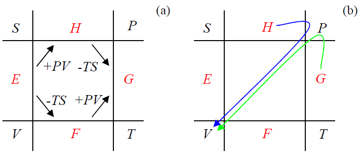
In this diagram, each thermodynamic potential is placed between its two canonical arguments – see Equation (???). The left two arrows in Figure 1.4.2a show the way the potentials H and F have been obtained from energy E – see Eqs. (???) and (???). This diagram hints that G has to be defined as shown by either of the two right arrows on that panel, i.e. as
G≡F+PV≡H−TS≡E−TS+PV.
In order to verify this idea, let us calculate the full differential of this new thermodynamic potential, using, e.g., the first form of Equation (???) together with Equation (???):
Gibbs energy: differential
dG=dF+d(PV)=(−SdT−PdV)+(PdV+VdP)≡−SdT+VdP,
so that if we know the function G(T,P), we can indeed readily calculate both entropy and volume:
S=−(∂G∂T)p,V=(∂G∂P)T.
Now I have to justify the collective name “thermodynamic potentials” used for E, H, F, and G. For that, let us consider an irreversible process, for example, a direct thermal contact of two bodies with different initial temperatures. As was discussed in Sec. 2, at such a process, the entropy may grow even without the external heat flow: dS≥0 at dQ=0 – see Equation (1.2.9). This means that at a more general process with dQ≠0, the entropy may grow faster than predicted by Equation (1.3.6), which has been derived for a reversible process, so that
dS≥dQT,
with the equality approached in the reversible limit. Plugging Equation (???) into Equation (1.3.5) (which, being just the energy conservation law, remains valid for irreversible processes as well), we get
dE≤TdS−PdV.
We can use this relation to have a look at the behavior of other thermodynamic potentials in irreversible situations, still keeping their definitions given by Eqs. (???), (???), and (???). Let us start from the (very common) case when both the temperature T and the volume V of a system are kept constant. If the process is reversible, then according to Equation (???), the full time derivative of the free energy F would equal zero. Equation (???) says that at an irreversible process, this is not necessarily so: if dT=dV=0, then
dFdt=ddt(E−TS)T=dEdt−TdSdt≤0.
Hence, in the general (irreversible) situation, F can only decrease, but not increase in time. This means that F eventually approaches its minimum value F(T,S), given by the equations of reversible thermodynamics. To re-phrase this important conclusion, in the case T= const, V= const, the free energy F, i.e. the difference E–TS, plays the role of the potential energy in the classical mechanics of dissipative processes: its minimum corresponds to the (in the case of F, thermodynamic) equilibrium of the system. This is one of the key results of thermodynamics, and I invite the reader to give it some thought. One of its possible handwaving interpretations of this fact is that the heat bath with fixed T>0, i.e. with a substantial thermal agitation of its components, “wants” to impose thermal disorder in the system immersed into it, by “rewarding” it with lower F for any increase of disorder.
Repeating the calculation for a different case, T= const, P= const, it is easy to see that in this case the same role is played by the Gibbs energy:
dGdt≡ddt(E−TS+PV)=dEdt−TdSdt+PdVdt≤(TdSdt−PdVdt)−TdSdt+PdVdt≡0
so that the thermal equilibrium now corresponds to the minimum of G rather than F.
For the two remaining thermodynamic potentials, E and H, the calculations similar to Eqs. (???) and (???) make less sense because that would require keeping S= const (with V= const for E, and P= const for H) for an irreversible process, but it is usually hard to prevent the entropy from growing if initially it had been lower than its equilibrium value, at least on the long-term basis.31 Thus the circular diagram is not so symmetric after all: G and F are somewhat more useful for most practical calculations than E and H.
Note that the difference G–F=PV between the two “more useful” potentials has very little to do with thermodynamics at all because this difference exists (although is not much advertised) in classical mechanics as well.32 Indeed, the difference may be generalized as G–F=–Fq, where q is a generalized coordinate, and F is the corresponding generalized force. The minimum of F corresponds to the equilibrium of an autonomous system (with F=0), while the equilibrium position of the same system under the action of external force F is given by the minimum of G. Thus the external force “wants” the system to subdue to its effect, “rewarding” it with lower G.
Moreover, the difference between F and G becomes a bit ambiguous (approach-dependent) when the product Fq may be partitioned into single-particle components – just as it is done in Eqs. (1.1.3) and (1.1.5) for the electric and magnetic fields. Here the applied field may be taken into account on the microscopic level, including its effect directly into the energy εk of each particle. In this case, the field contributes to the total internal energy E directly, and hence the thermodynamic equilibrium (at T= const) is described as the minimum of F. (We may say that in this case F=G, unless a difference between these thermodynamic potentials is created by the actual mechanical pressure P.) However, in some cases, typically for condensed systems, with their strong interparticle interactions, the easier (and sometimes the only one practicable33) way to account for the field is on the macroscopic level, taking G=F–Fq. In this case, the same equilibrium state is described as the minimum of G. (Several examples of this dichotomy will be given later in this course.) Whatever the choice, one should mind not take the same field effect into account twice.
One more important conceptual question I would like to discuss here is why usually statistical physics pursues the calculation of thermodynamic potentials, rather than just of a relation between P, V, and T. (Such relation is called the equation of state of the system.) Let us explore this issue on the particular but important example of an ideal classical gas in thermodynamic equilibrium, for which the equation of state should be well known to the reader from undergraduate physics:34
Ideal gas: equation of state
PV=NT,
where N is the number of particles in volume V. (In Chapter 3, we will derive Equation (???) from statistics.) Let us try to use it for the calculation of all thermodynamic potentials, and all other thermodynamic variables discussed above. We may start, for example, from the calculation of the free energy F. Indeed, integrating the second of Eqs. (???) with the pressure calculated from Equation (???), P = NT/V, we get
F=-\left.\int P d V\right|_{T=\mathrm{const}}=-N T \int \frac{d V}{V} \equiv-N T \int \frac{d(V / N)}{(V / N)}=-N T \ln \frac{V}{N}+N f(T) \label{45}
where V has been divided by N in both instances just to represent F as a manifestly extensive variable, in this uniform system proportional to N. The integration “constant” f(T) is some function of temperature, which cannot be recovered from the equation of state. This function affects all other thermodynamic potentials, and the entropy as well. Indeed, using the first of Eqs. (\ref{35}) together with Equation (\ref{45}), we get
S = -\left(\frac{\partial F}{\partial T} \right)_V = N \left[ \ln \frac{V}{N} - \frac{df(T)}{dT} \right], \label{46}
and now may combine Eqs. (\ref{33}) with (\ref{46}) to calculate the (internal) energy of the gas,35
E=F+T S=\left[-N T \ln \frac{V}{N}+N f(T)\right]+T\left[N \ln \frac{V}{N}-N \frac{d f(T)}{d T}\right] \equiv N\left[f(T)-T \frac{d f(T)}{d T}\right], \label{47}
then use Eqs. (\ref{27}), (\ref{44}) and (\ref{47}) to calculate its enthalpy,
H = E + PV = E + NT = N \left[f(T)-T \frac{d f(T)}{d T} + T \right], \label{48}
and, finally, plug Eqs. (\ref{44}) and (\ref{45}) into Equation (\ref{37}) to calculate the Gibbs energy
G = F + PV = N\left[ -T \ln \frac{V}{N} + f(T) + T \right]. \label{49}
One might ask whether the function f(T) is physically significant, or it is something like the inconsequential, arbitrary constant – like the one that may be always added to the potential energy in non-relativistic mechanics. In order to address this issue, let us calculate, from Eqs. (\ref{24}) and (\ref{28}), both heat capacities, which are evidently measurable quantities:
C_{V}=\left(\frac{\partial E}{\partial T}\right)_{V}=-N T \frac{d^{2} f}{d T^{2}}, \label{50}
C_{P}=\left(\frac{\partial H}{\partial T}\right)_{P}=N\left(-T \frac{d^{2} f}{d T^{2}}+1\right)=C_{V}+N .\label{51}
We see that the function f(T), or at least its second derivative, is measurable.36 (In Chapter 3, we will calculate this function for two simple “microscopic” models of the ideal classical gas.) The meaning of this function is evident from the physical picture of the ideal gas: the pressure P exerted on the walls of the containing volume is produced only by the translational motion of the gas molecules, while their internal energy E (and hence other thermodynamic potentials) may be also contributed by the internal dynamics of the molecules – their rotations, vibrations, etc. Thus, the equation of state does not give us the full thermodynamic description of a system, while the thermodynamic potentials do.