2.4: Canonical ensemble and the Gibbs distribution

As was shown in Sec. 2 (see also a few problems of the list given in the end of this chapter), the microcanonical distribution may be directly used for solving some simple problems. However, its further development, also due to J. Gibbs, turns out to be much more convenient for calculations.

Let us consider a statistical ensemble of macroscopically similar systems, each in thermal equilibrium with a heat bath of the same temperature $T$ (Figure $\PageIndex{1a}$). Such an ensemble is called canonical.

Figure $\PageIndex{1}$: (a) A system in a heat bath (i.e. a canonical ensemble’s member) and (b) the energy spectrum of the composite system (including the heat bath).

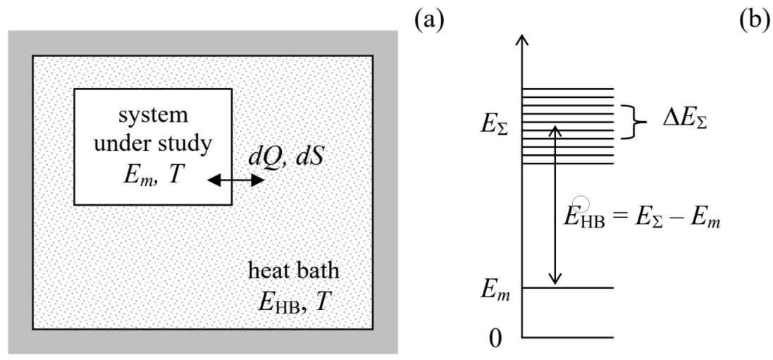
It is intuitively evident that if the heat bath is sufficiently large, any thermodynamic variables characterizing the system under study should not depend on the heat bath’s environment. In particular, we may assume that the heat bath is thermally insulated, so that the total energy $E_{\Sigma}$ of the composite system, consisting of the system of our interest plus the heat bath, does not change in time. For example, if the system of our interest is in a certain (say, $m^{th}$) quantum state, then the sum

$$E_{\Sigma} = E_m + E_{HB} \label{52}$$

is time-independent. Now let us partition the considered canonical ensemble of such systems into much smaller sub-ensembles, each being a microcanonical ensemble of composite systems whose total, time independent energies $E_{\Sigma}$ are the same – as was discussed in Sec. 2, within a certain small energy interval $\Delta E_{\Sigma} << E_{\Sigma}$ – see Figure $\PageIndex{1b}$. Due to the very large size of each heat bath in comparison with that of the system under study, the heat bath’s density of states $g_{HB}$ is very high, and $\Delta E_{\Sigma}$ may be selected so that

$$\frac{1}{g_{HB}} << \Delta E_{\Sigma} << | E_m - E_{m'}| <<E_{HB}, \label{53}$$

where $m$ and $m’$ are any states of the system of our interest.

According to the microcanonical distribution, the probabilities to find the composite system, within each of these microcanonical sub-ensembles, in any state are equal. Still, the heat bath energies $E_{HB} = E_{\Sigma} – E_m$ (Figure $\PageIndex{1b}$) of the members of this sub-ensemble may be different – due to the difference in $E_m$. The probability $W(E_m)$ to find the system of our interest (within the selected sub-ensemble) in a state with energy $E_m$ is proportional to the number $\Delta M$ of the corresponding heat baths in the sub-ensemble. As Figure $\PageIndex{1b}$ shows, in this case we may write $\Delta M = g_{HB}(E_{HB})\Delta E_{\Sigma}$. As a result, within the microcanonical sub-ensemble with the total energy $E_{\Sigma}$,

$$W_m \propto \Delta M = g_{HB} ( E_{HB}) \Delta E_{\Sigma} = g_{HB} (E_{\Sigma} − E_m ) \Delta E_{\Sigma} . \label{54}$$

Let us simplify this expression further, using the Taylor expansion with respect to relatively small $E_m << E_{\Sigma}$. However, here we should be careful. As we have seen in Sec. 2, the density of states of a large system is an extremely fast growing function of energy, so that if we applied the Taylor expansion directly to Equation ($\ref{54}$), the Taylor series would converge for very small $E_m$ only. A much broader applicability range may be obtained by taking logarithms of both parts of Equation ($\ref{54}$) first:

$$\ln W_m = \text{ const } + \ln [ g_{HB} (E_{\Sigma} − E_m)] + \ln \Delta E_{\Sigma} = \text{ const } + S_{HB} (E_{\Sigma} − E_m ), \label{55}$$

where the last equality results from the application of Equation ($2.2.18$) to the heat bath, and $\ln \Delta E_{\Sigma}$ has been incorporated into the (inconsequential) constant. Now, we can Taylor-expand the (much more smooth) function of energy on the right-hand side, and limit ourselves to the two leading terms of the series:

$$\ln W_m \approx \text{ const } + S_{HB} \left|_{E_m = 0} - \frac{dS_{HB}}{dE_{HB}}\right|_{E_m =0} E_m. \label{56}$$

But according to Equation ($1.2.6$), the derivative participating in this expression is nothing else than the reciprocal temperature of the heat bath, which (due to the large bath size) does not depend on whether $E_m$ is equal to zero or not. Since our system of interest is in the thermal equilibrium with the bath, this is also the temperature $T$ of the system – see Equation ($1.2.5$). Hence Equation ($\ref{56}$) is merely

$$\ln W_m = \text{ const } − \frac{E_m}{T}. \label{57}$$

This equality describes a substantial decrease of $W_m$ as $E_m$ is increased by $\sim T$, and hence our linear approximation ($\ref{56}$) is virtually exact as soon as $E_{HB}$ is much larger than $T$ – the condition that is rather easy to satisfy, because as we have seen in Sec. 2, the average energy per one degree of freedom of the system of the heat bath is also of the order of $T$, so that its total energy is much larger because of its much larger size.

Now we should be careful again because so far Equation ($\ref{57}$) was only derived for a sub-ensemble with a certain fixed $E_{\Sigma}$. However, since the second term on the right-hand side of Equation ($\ref{57}$) includes only $E_m$ and $T$, which are independent of $E_{\Sigma}$, this relation, perhaps with different constant terms, is valid for all sub-ensembles of the canonical ensemble, and hence for that ensemble as the whole. Hence for the total probability to find our system of interest in a state with energy $E_m$, in the canonical ensemble with temperature $T$, we can write

Gibbs distribution:

$$\boxed{ W_m = \text{ const} \times \text{exp}\left\{ - \frac{E_m}{T} \right\} \equiv \frac{1}{Z} \text{exp}\left\{-\frac{E_m}{T}\right\}.} \label{58}$$

This is the famous Gibbs distribution,³⁶ sometimes called the “canonical distribution”, which is arguably the summit of statistical physics,³⁷ because it may be used for a straightforward (or at least conceptually straightforward :-) calculation of all statistical and thermodynamic variables of a vast range of systems.

Before illustrating this, let us first calculate the coefficient $Z$ participating in Equation ($\ref{58}$) for the general case. Requiring, per Equation ($2.1.4$), the sum of all $W_m$ to be equal 1, we get

Statistical sum:

$$\boxed{ Z = \sum_m \text{exp}\left\{-\frac{E_m}{T}\right\},} \label{59}$$

where the summation is formally extended to all quantum states of the system, though in practical calculations, the sum may be truncated to include only the states that are noticeably occupied. The apparently humble normalization coefficient $Z$ turns out to be so important for applications that it has a special name – or actually, two names: either the statistical sum or the partition function of the system. To appreciate the importance of $Z$, let us use the general expression ($2.2.11$) for entropy to calculate it for the particular case of the canonical ensemble, i.e. the Gibbs distribution ($\ref{58}$) of the probabilities $W_n$:

$$S = -\sum_m W_m \ln W_m = \frac{\ln Z}{Z} \sum_m \text{exp}\left\{-\frac{E_m}{T}\right\} + \frac{1}{ZT} \sum_m E_m \text{exp}\left\{-\frac{E_m}{T}\right\}. \label{60}$$

On the other hand, according to the general rule ($2.1.7$), the thermodynamic (i.e. ensemble-averaged) value $E$ of the internal energy of the system is

$$E = \sum_m W_mE_m = \frac{1}{Z} \sum_m E_m \text{exp}\left\{-\frac{E_m}{T}\right\}, \label{61a}$$

so that the second term on the right-hand side of Equation ($\ref{60}$) is just $E/T$, while the first term equals $\ln Z$, due to Equation ($\ref{59}$). (By the way, using the notion of reciprocal temperature $\beta \equiv 1/T$, with the account of Equation ($\ref{59}$), Equation ($\ref{61a}$) may be also rewritten as

$\mathbf{E}$ from $\mathbf{Z}$:

$$\boxed{ E = - \frac{\partial (\ln Z)}{\partial \beta}.} \label{61b}$$

This formula is very convenient for calculations if our prime interest is the average internal energy $E$ rather than $F$ or $W_n$.) With these substitutions, Equation ($\ref{60}$) yields a very simple relation between the statistical sum and the entropy of the system:

$$S = \frac{E}{T}+\ln Z. \label{62}$$

Now using Equation ($1.4.10$), we see that Equation ($\ref{62}$) gives a straightforward way to calculate the free energy $F$ of the system from nothing other than its statistical sum (and temperature):

$\mathbf{F}$ from $\mathbf{Z}$:

$$\boxed{F \equiv E −TS = −T \ln Z.} \label{63}$$

The relations ($\ref{61b}$) and ($\ref{63}$) play the key role in the connection of statistics to thermodynamics, because they enable the calculation, from $Z$ alone, of the thermodynamic potentials of the system in equilibrium, and hence of all other variables of interest, using the general thermodynamic relations – see especially the circular diagram shown in Figure $1.4.2$, and its discussion in Sec. 1.4. Let me only note that to calculate the pressure $P$, e.g., from the second of Eqs. ($1.4.12$), we would need to know the explicit dependence of $F$, and hence of the statistical sum $Z$ on the system’s volume $V$. This would require the calculation, by appropriate methods of either classical or quantum mechanics, of the dependence of the eigenenergies $E_m$ on the volume. Numerous examples of such calculations will be given later in the course.

Before proceeding to first such examples, let us notice that Eqs. ($\ref{59}$) and ($\ref{63}$) may be readily combined to give an elegant equality,

$$\text{exp}\left\{-\frac{F}{T}\right\} = \sum_m \text{exp}\left\{-\frac{E_m}{T}\right\}. \label{64}$$

This equality, together with Equation ($\ref{59}$), enables us to rewrite the Gibbs distribution ($\ref{58}$) in another form:

$$W_m = \text{exp}\left\{-\frac{F - E_m}{T}\right\}, \label{65}$$

more convenient for some applications. In particular, this expression shows that since all probabilities $W_m$ are below 1, $F$ is always lower than the lowest energy level. Also, Equation ($\ref{65}$) clearly shows that the probabilities $W_m$ do not depend on the energy reference, i. e. on an arbitrary constant added to all $E_m$ – and hence to $E$ and $F$.