5.4: Fluctuations as functions of time

In the previous sections, the averaging \(\langle ...\rangle\) of any function was assumed to be over an appropriate statistical ensemble of many similar systems. However, as was discussed in Sec. 2.1, most physical systems of interest are ergodic. If such a system is also stationary, i.e. the statistical averages of its variables do not change with time, the averaging may be also understood as that over a sufficiently long time interval. In this case, we may think about fluctuations of any variable \(f\) as of a random process taking place in just one system, but developing in time: \(\tilde{f} = \tilde{f}(t)\).

There are two mathematically equivalent approaches to the description of such random functions of time, called the time-domain picture and the frequency-domain picture, their relative convenience depending on the particular problem to be solved. In the time domain, we need to characterize a random fluctuation \(\tilde{f} (t)\) by some deterministic function of time. Evidently, the average \(\langle \tilde{f}(t)\rangle\) cannot be used for this purpose, because it equals zero – see Equation (\(5.1.2\)). Of course, the variance (\(5.1.3\)) does not equal zero, but if the system is stationary, that average cannot depend on time either. Because of that, let us consider the following average:

\[\langle \tilde{f}(t)\tilde{f}(t')\rangle . \label{46}\]

Generally, this is a function of two arguments. However, in a stationary system, the average like (\ref{46}) may depend only on the difference,

\[ \tau \equiv t' − t , \label{47}\]

between the two observation times. In this case, the average (\ref{46}) is called the correlation function of the variable \(f\):

Correlation function:

\[\boxed{ K_f (\tau ) \equiv \langle \tilde{f}(t) \tilde{f}(t+\tau ) \rangle. } \label{48}\]

Again, here the averaging may be understood as that either over a statistical ensemble of macroscopically similar systems or over a sufficiently long interval of the time argument \(t\), with the argument \(\tau\) kept constant. The correlation function's name¹⁵ catches the idea of this notion very well: \(K_f(\tau )\) characterizes the mutual relation between the fluctuations of the variable \(f\) at two times separated by the given interval \(\tau \). Let us list the basic properties of this function.¹⁶

First of all, \(K_f (\tau )\) has to be an even function of the time delay \(\tau \). Indeed, we may write

\[ K_f (-\tau ) = \langle \tilde{f}(t) \tilde{f}(t-\tau ) \rangle \equiv \langle \tilde{f}(t-\tau ) \tilde{f}(t) \rangle = \langle \tilde{f}(t') \tilde{f}(t'+\tau ) \rangle , \label{49}\]

with \(t' \equiv t – \tau \). For stationary processes, this average cannot depend on the common shift of two observation times, so that the averages (\ref{48}) and (\ref{49}) have to be equal:

\[K_f (-\tau ) = K_f (\tau ). \label{50}\]

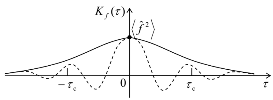
Second, at \(\tau \rightarrow 0\) the correlation function tends to the variance:

\[K_f (0) = \langle \tilde{f}(t)\tilde{f}(t)\rangle = \langle \tilde{f}^2 \rangle \geq 0. \label{51}\]

In the opposite limit, when \(\tau\) is much larger than certain characteristic correlation time \(\tau_c\) of the system,¹⁷ the correlation function has to tend to zero because the fluctuations separated by such time interval are virtually independent (uncorrelated). As a result, the correlation function typically looks like one of the plots sketched in Figure \(\PageIndex{1}\).

Figure \(\PageIndex{1}\): The correlation function of fluctuations: two typical examples.

Note that on a time scale much longer than \(\tau_c\), any physically-realistic correlation function may be well approximated with a delta function of \(\tau \). (For example, for a process which is a sum of independent very short pulses, e.g., the gas pressure force exerted on the container wall (Figure \(5.3.1\)), such approximation is legitimate on time scales much longer than the single pulse duration, e.g., the time of particle's interaction with on the wall at the impact.)

\[\tilde{f} (t) = \int^{+ \infty}_{- \infty} f_{\omega} e^{-i\omega t} d\omega , \label{52}\]

with the reciprocal transform being

\[f_{\omega} = \frac{1}{2 \pi } \int^{+\infty}_{-\infty} \tilde{f}(t) e^{i \omega t} dt. \label{53}\]

If the function \(\tilde{f} (t)\) is random (as it is in the case of fluctuations), with zero average, its Fourier transform \(f_{\omega}\) is also a random function (now of frequency), also with a vanishing statistical average. Indeed, now thinking of the operation \(\langle ...\rangle\) as an ensemble averaging, we may write

\[\langle f_{\omega} \rangle = \left\langle \frac{1}{2\pi} \int^{+\infty}_{-\infty} \tilde{f}(t) e^{i\omega t} dt \right\rangle = \frac{1}{2\pi} \int^{+\infty}_{-\infty} \langle \tilde{f}(t)\rangle e^{i\omega t} dt = 0 . \label{54}\]

The simplest non-zero average may be formed similarly to Equation (\ref{46}), but with due respect to the complex-variable character of the Fourier images:

\[\left\langle f_{\omega}f_{\omega'}^* \right\rangle = \langle \frac{1}{(2\pi )^2} \int^{+\infty}_{-\infty} dt' \int^{+\infty}_{-\infty} dt \langle \tilde{f}(t) \tilde{f} (t') \rangle e^{i(\omega' t' - \omega t)}. \label{55}\]

It turns out that for a stationary process, the averages (\ref{46}) and (\ref{55}) are directly related. Indeed, since the integration over \(t'\) in Equation (\ref{55}) is in infinite limits, we may replace it with the integration over \(\tau \equiv t' – t\) (at fixed \(t\)), also in infinite limits. Replacing \(t'\) with \(t + \tau\) in the expressions under the integral, we see that the average is just the correlation function \(K_f(\tau )\), while the time exponent is equal to \(\exp \{i(\omega ' – \omega )t\}\exp\{i\omega '\tau \}\). As a result, changing the order of integration, we get

\[\left\langle f_{\omega} f_{\omega^{\prime}}^{*}\right\rangle=\frac{1}{(2 \pi)^{2}} \int_{-\infty}^{+\infty} d t \int_{-\infty}^{+\infty} d \tau K_{f}(\tau) e^{i\left(\omega-\omega^{\prime}\right) t} e^{i \omega^{\prime} \tau} \equiv \frac{1}{(2 \pi)^{2}} \int_{-\infty}^{+\infty} K_{f}(\tau) e^{i \omega^{\prime} \tau} d \tau \int_{-\infty}^{+\infty} e^{i\left(\omega-\omega^{\prime}\right) t} d t . \label{56}\]

But the last integral is just \(2\pi \delta (\omega – \omega')\),¹⁹ so that we finally get

\[\left\langle f_{\omega} f_{\omega^{\prime}}^{*}\right\rangle= S_f ( \omega ) \delta (\omega - \omega' ), \label{57}\]

where the real function of frequency,

Spectral density of fluctuations:

\[\boxed{ S_f ( \omega ) \equiv \frac{1}{2\pi } \int^{+\infty}_{-\infty} K_f (\tau ) e^{i\omega \tau} d \tau = \frac{1}{\pi} \int^{\infty}_0 K_f (\tau ) \cos \omega \tau d \tau , } \label{58}\]

Wiener-Khinchin theorem:

\[\boxed{ K_f (\tau ) = \int^{+\infty}_{-\infty} S_f (\omega ) e^{-i \omega \tau} d \omega = 2 \int^{\infty}_0 S_f (\omega ) \cos \omega \tau d \omega . } \label{59}\]

In particular, for the fluctuation variance, Equation (\ref{59}) yields

\[\langle \tilde{f}^2 \rangle \equiv K_f (0) = \int^{+\infty}_{-\infty} S_f (\omega ) d\omega \equiv 2 \int^{\infty}_0 S_f ( \omega ) d \omega . \label{60}\]

The last relation shows that the term “spectral density” describes the physical sense of the function \(S_f(\omega )\) very well. Indeed, if a random signal \(f(t)\) had been passed through a frequency filter with a small bandwidth \(\Delta \nu << \nu \) of positive cyclic frequencies, the integral in the last form of Equation (\ref{60}) could be limited to the interval \(\Delta \omega = 2\pi \Delta \nu \), i.e. the variance of the filtered signal would become

\[\left\langle \tilde{f}^2 \right\rangle_{\Delta \nu} = 2S_f (\omega ) \Delta \omega \equiv 4 \pi S_f ( \omega ) \Delta \nu . \label{61}\]

(A popular alternative definition of the spectral density is \(\mathscr{S}_f(\nu ) \equiv 4\pi S_f(\omega )\), making the average (\ref{61}) equal to just \(\mathscr{S}_f(\nu )\Delta \nu \).)

To conclude this introductory (mostly mathematical) section, let me note an important particular case. If the spectral density of some process is nearly constant within all the frequency range of interest, \(S_f(\omega ) =\) const \(= S_f(0)\),²² Equation (\ref{59}) shows that its correlation function may be well approximated with a delta function:

\[K_f ( \tau ) = S_f (0) \int^{+\infty}_{-\infty} e^{-i\omega \tau}d\omega = 2\pi S_f (0) \delta (\tau). \label{62}\]

From this relation stems another popular name of the white noise, the delta-correlated process. We have already seen that this is a very reasonable approximation, for example, for the gas pressure force fluctuations (Figure \(5.3.1\)). Of course, for the spectral density of a realistic, limited physical variable the approximation of constant spectral density cannot be true for all frequencies (otherwise, for example, the integral (\ref{60}) would diverge, giving an unphysical, infinite value of its variance), and may be valid only at frequencies much lower than \(1/\tau_c\).