5.5: Fluctuations and Dissipation

One more important assumption of this theory is that the system's motion does not violate the thermal equilibrium of the environment – well fulfilled in many cases. (Think, for example, about a typical mechanical pendulum – its motion does not overheat the air around it to any noticeable extent.) In this case, the averaging over a statistical ensemble of similar environments, at a fixed, specific motion of the system of interest, may be performed assuming their thermal equilibrium.²⁴ I will denote such a “primary” averaging by the usual angle brackets \(\langle ...\rangle \). At a later stage, we may carry out additional, “secondary” averaging, over an ensemble of many similar systems of interest, coupled to similar environments. When we do, such double averaging will be denoted by double angle brackets \(\langle \langle ...\rangle \rangle \).

Let me start from a simple classical system, a 1D harmonic oscillator whose equation of evolution may be represented as

\[m\ddot{q} + \kappa q = \mathscr{F}_{det}(t) + \mathscr{F}_{env}(t) \equiv \mathscr{F}_{det}(t)+\langle \mathscr{F} \rangle + \tilde{\mathscr{F}}(t), \quad \text{ with } \langle \tilde{\mathscr{F}}(t) \rangle = 0, \label{63}\]

where \(q\) is the (generalized) coordinate of the oscillator, \(\mathscr{F}_{det}(t)\) is the deterministic external force, while both components of the force \(\mathscr{F}_{env}(t)\) represent the impact of the environment on the oscillator's motion. Again, on the time scale of the fast-moving environmental components, the oscillator's motion is slow. The average component \(\langle F \rangle\) of the force exerted by the environment on such a slowly moving object is frequently independent of its coordinate \(q\) but does depend on its velocity \(\dot{q} \). For most such systems, the Taylor expansion of the force in small velocity has a non-zero linear term:

\[\langle \mathscr{F} \rangle = −\eta \dot{q} , \label{64}\]

where the constant \(\eta\) is usually called the drag (or “kinematic friction”, or “damping”) coefficient, so that Equation (\ref{63}) may be rewritten as

Langevin equation for classical oscillator:

\[\boxed{ m \ddot{q} + \eta \dot{q} + \kappa q = \mathscr{F}_{det} (t) + \tilde{\mathscr{F}}(t).} \label{65}\]

Plugging into Equation (\ref{65}) the representation of both variables in the Fourier form similar to Equation (\(5.4.7\)), and requiring the coefficients before the same \(\exp\{-i\omega t\}\) to be equal on both sides of the equation, for their Fourier images we get the following relation:

\[ − m \omega^2 q_{\omega} − i \omega \eta q_{\omega} + \kappa q_{\omega} =\mathscr{F}_{\omega} , \label{66}\]

which immediately gives us \(q_{\omega }\), i.e. the (random) complex amplitude of the coordinate fluctuations:

\[q_{\omega} = \frac{\mathscr{F}_{\omega}}{(\kappa - m\omega^2) - i \eta \omega} \equiv \frac{\mathscr{F}_{\omega}}{m(\omega^2_0 - \omega^2 ) - i \eta \omega}. \label{67}\]

\[S_q (w) = \frac{1}{m^2 (\omega^2_0 - \omega^2)^2 + \eta^2 \omega^2} S_{\mathscr{F}} ( \omega ). \label{68}\]

In the so-called low-damping limit (\(\eta << m\omega_0\)), the fraction on the right-hand side of Equation (\ref{68}) has a sharp peak near the oscillator's own frequency \(\omega_0\) (describing the well-known effect of high-\(Q\) resonance), and may be well approximated in that vicinity as

\[\frac{1}{m^2(\omega^2_0 - \omega^2)^2 + (\eta \omega )^2} \approx \frac{1}{\eta^2 \omega^2_0 (\xi^2 + 1)}, \quad \text{ with } \xi \equiv \frac{2m(\omega - \omega_0 )}{\eta}. \label{69}\]

\[\langle\langle \tilde{q}^2\rangle\rangle = 2\int^{\infty}_0 S_q (\omega ) d \omega \approx 2 \int_{\omega \approx \omega_0} S_q (\omega ) d\omega = 2S_{\mathscr{F}}(\omega_0) \frac{1}{\eta^2 \omega^2_0} \frac{\eta}{2m} \int^{+\infty}_{-\infty} \frac{d\xi}{\xi^2 +1} . \label{70}\]

This is a well-known table integral,³¹ equal to \(\pi \), so that, finally:

\[\langle\langle \tilde{q}^2\rangle\rangle = 2S_{\mathscr{F}} (\omega_0 ) \frac{1}{\eta^2 \omega^2_0} \frac{\eta}{2m} \pi \equiv \frac{\pi}{m\omega^2_0 \eta} S_{\mathscr{F}} (\omega_0) \equiv \frac{\pi}{\kappa \eta} S_{\mathscr{F}}(\omega_0). \label{71}\]

But on the other hand, the weak interaction with the environment should keep the oscillator in thermodynamic equilibrium at the same temperature \(T\). Since our analysis has been based on the classical Langevin equation (\ref{65}), we may only use it in the classical limit \(\hbar \omega_0 << T\), in which we may use the equipartition theorem (\(2.2.30\)). In our current notation, it yields

\[\frac{\kappa}{2} \langle \langle \tilde{q}^2 \rangle \rangle = \frac{T}{2}. \label{72}\]

Comparing Eqs. (\ref{71}) and (\ref{72}), we see that the spectral density of the random force exerted by the environment has to be fundamentally related to the damping it provides:

\[S_{\mathscr{F}} ( \omega_0 ) = \frac{\eta}{\pi} T. \label{73a}\]

Now we may argue (rather convincingly :-) that since this relation does not depend on oscillator's parameters \(m\) and \(\kappa \), and hence its eigenfrequency \(\omega_0 = (\kappa /m)^{1/2}\), it should be valid at any relatively low frequency \((\omega \tau_c << 1)\). Using Equation (\(5.4.13\)) with \(\omega \rightarrow 0\), it may be also rewritten as a formula for the effective low-frequency drag coefficient:

No dissipation without fluctuations:

\[\boxed{\eta = \frac{1}{T} \int^{\infty}_0 K_{\mathscr{F}} (\tau ) d\tau \equiv \frac{1}{T} \int^{\infty}_0 \langle \tilde{\mathscr{F}}(0) \tilde{\mathscr{F}}(\tau)\rangle d\tau .} \label{73b}\]

Formulas (\ref{73a}-\ref{73b}) reveal an intimate, fundamental relation between the fluctuations and the dissipation provided by a thermally-equilibrium environment. Parroting the famous political slogan, there is “no dissipation without fluctuation” – and vice versa. This means in particular that the phenomenological description of dissipation barely by the drag force in classical mechanics³² is (approximately) valid only when the energy scale of the process is much larger than \(T\). To the best of my knowledge, this fact was first recognized in 1905 by A. Einstein,³³ for the following particular case.

Let us apply our result (\ref{73a}-\ref{73b}) to a free 1D Brownian particle, by taking \(\kappa = 0\) and \(\mathscr{F}_{det}(t) = 0\). In this case, both relations (\ref{71}) and (\ref{72}) give infinities. To understand the reason for that divergence, let us go back to the Langevin equation (\ref{65}) with not only \(\kappa = 0\) and \(\mathscr{F}_{det}(t)= 0\), but also \(m \rightarrow 0\) – just for the sake of simplicity. (The latter approximation, frequently called the overdamping limit, is quite appropriate, for example, for the motion of small particles in viscous fluids – such as in R. Brown's experiments.) In this approximation, Equation (\ref{65}) is reduced to a simple equation,

\[\eta \dot{q} = \tilde{\mathscr{F}} (t), \quad \text{ with } \langle \tilde{\mathscr{F}}(t)\rangle =0 , \label{74}\]

which may be readily integrated to give the particle's displacement during a finite time interval \(t\):

\[\Delta q(t) \equiv q(t) - q(0) = \frac{1}{\eta} \int^t_0 \tilde{\mathscr{F}} (t') dt'. \label{75}\]

Evidently, at the full statistical averaging of the displacement, the fluctuation effects vanish, but this does not mean that the particle does not move – just that it has equal probabilities to be shifted in either of two possible directions. To see that, let us calculate the variance of the displacement:

\[\left\langle\left\langle\Delta \tilde{q}^{2}(t)\right\rangle\right)=\frac{1}{\eta^{2}} \int_{0}^{t} d t^{\prime} \int_{0}^{t} d t^{\prime \prime}\left(\widetilde{\mathscr{F}}\left(t^{\prime}\right), \widetilde{\mathscr{F}}\left(t^{\prime \prime}\right)\right\rangle \equiv \frac{1}{\eta^{2}} \int_{0}^{t} d t^{\prime} \int_{0}^{t} d t^{\prime \prime} K_{\mathscr{F}}\left(t^{\prime}-t^{\prime \prime}\right). \label{76} \]

As we already know, at times \(\tau >> \tau_c\), the correlation function may be well approximated by the delta function – see Equation (\(5.4.17\)). In this approximation, with \(S_{\mathscr{F}}(0)\) expressed by Equation (\ref{73a}), we get

\[\left\langle\left\langle\Delta \widetilde{q}^{2}(t)\right\rangle\right\rangle=\frac{2 \pi}{\eta^{2}} S_{\mathscr{F}}(0) \int_{0}^{t} d t^{\prime} \int_{0}^{\prime} d t^{\prime \prime} \delta\left(t^{\prime \prime}-t^{\prime}\right)=\frac{2 \pi}{\eta^{2}} \frac{\eta T}{\pi} \int_{0}^{t} d t^{\prime}=\frac{2 T}{\eta} t \equiv 2 D t, \label{77}\]

with

Einstein's relation:

\[ \boxed{D = \frac{T}{\eta}.} \label{78}\]

The final form of Equation (\ref{77}) describes the well-known law of diffusion (“random walk”) of a 1D system, with the r.m.s. deviation from the point of origin growing as \((2Dt)^{1/2}\). The coefficient \(D\) is this relation is called the coefficient of diffusion, and Equation (\ref{78}) describes the extremely simple and important³⁴ Einstein's relation between that coefficient and the drag coefficient. Often this relation is rewritten, in the SI units of temperature, as \(D = \mu k_BT_K\), where \(\mu \equiv 1/\eta\) is the mobility of the particle. The physical sense of \(\mu\) becomes clear from the expression for the deterministic velocity (particle's “drift”), which follows from the averaging of both sides of Equation (\ref{74}) after the restoration of the term \(\mathscr{F}_{det}(t)\) in it:

\[\nu_{drift} \equiv \langle \langle \dot{q}(t)\rangle\rangle = \frac{1}{\eta} \mathscr{F}_{det}(t) \equiv \mu \mathscr{F}_{det}(t), \label{79}\]

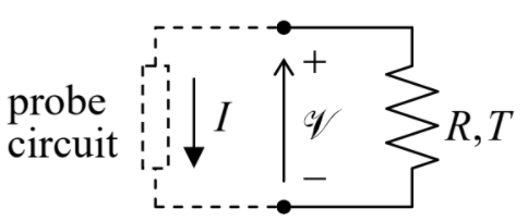
Another famous embodiment of the general Equation (\ref{73a}-\ref{73b}) is the thermal (or “Johnson”, or “Johnson Nyquist”, or just “Nyquist”) noise in resistive electron devices. Let us consider a two-terminal, dissipation-free “probe” circuit, playing the role of the harmonic oscillator in our analysis carried out above, connected to a resistive device (Figure \(\PageIndex{1}\)), playing the role of the probe circuit's environment. (The noise is generated by the thermal motion of numerous electrons, randomly moving inside the resistive device.) For this system, one convenient choice of the conjugate variables (the generalized coordinate and generalized force) is, respectively, the electric charge \(Q \equiv \int I(t)dt\) that has passed through the “probe” circuit by time \(t\), and the voltage \(\mathscr{V}\) across its terminals, with the polarity shown in Figure \(\PageIndex{1}\). (Indeed, the product \(\mathscr{V}dQ\) is the elementary work \(d\mathscr{W}\) done by the environment on the probe circuit.)

Figure \(\PageIndex{1}\): A resistive device as a dissipative environment of a two-terminal probe circuit.

Making the corresponding replacements, \(q \rightarrow Q\) and \(\mathscr{F} \rightarrow \mathscr{V}\) in Equation (\ref{64}), we see that it becomes

\[\langle \mathscr{V} \rangle = -\eta \dot{Q} \equiv - \eta I. \label{80}\]

Comparing this relation with Ohm's law, \(\mathscr{V} = R(-I)\),³⁶ we see that in this case, the coefficient \(\eta\) has the physical sense of the usual Ohmic resistance \(R\) of our dissipative device,³⁷ so that Equation (\ref{73a}) becomes

\[S_{\mathscr{V}} (\omega ) = \frac{R}{\pi}T. \label{81a}\]

Using last equality in Equation (\(5.4.16\)), and transferring to the SI units of temperature (\(T = k_BT_K\)), we may bring this famous Nyquist formula³⁸ to its most popular form:

Nyquist formula:

\[\boxed{\left\langle \tilde{\mathscr{V}}^2 \right\rangle_{\Delta \nu} = 4k_BT_K R \Delta \nu. } \label{81b}\]

Note that according to Equation (\ref{65}), this result is only valid at a negligible speed of change of the coordinate \(q\) (in our current case, negligible current \(I\)), i.e. Equation (\ref{81a}-\ref{81c}) expresses the voltage fluctuations as would be measured by a virtually ideal voltmeter, with its input resistance much higher than \(R\).

On the other hand, using a different choice of generalized coordinate and force, \(q \rightarrow \Phi \), \(\mathscr{F} \rightarrow I\) (where \(\Phi \equiv \int \mathscr{V}(t)dt\) is the generalized magnetic flux, so that \(d\mathscr{W} = I\mathscr{V}(t)dt \equiv Id\Phi \)), we get \(\eta \rightarrow 1/R\), and Equation (\ref{73a}-\ref{73b}) yields the thermal fluctuations of the current through the resistive device, as measured by a virtually ideal ammeter, i.e. at \(\mathscr{V} \rightarrow 0\):

\[S_I (\omega ) = \frac{1}{\pi R} T, \quad \text{ i.e. } \left\langle \tilde{I}^2 \right\rangle_{\Delta \nu} = \frac{4k_BT_K}{R} \Delta \nu . \label{81c}\]

The nature of Eqs. (\ref{81a}-\ref{81c}) is so fundamental that they may be used, in particular, for the so-called Johnson noise thermometry.³⁹ Note, however, that these relations are valid for noise in thermal equilibrium only. In electric circuits that may be readily driven out of equilibrium by an applied voltage \(\mathscr{V}\), other types of noise are frequently important, notably the shot noise, which arises in short conductors, e.g., tunnel junctions, at applied voltages with \(|\mathscr{V} | >> T /q\), due to the discreteness of charge carriers.⁴⁰ A straightforward analysis (left for the reader's exercise) shows that this noise may be characterized by current fluctuations with the following low-frequency spectral density:

Schottky formula:

\[ \boxed{ S_I (\omega ) = \frac{\left| q \tilde{I}\right|}{2\pi}, \quad \text{ i.e. } \left\langle \tilde{I}^2 \right\rangle_{\Delta \nu} = 2 \left| q \tilde{I} \right\rangle \Delta \nu , } \label{82}\]

where \(q\) is the electric charge of a single current carrier. This is the Schottky formula,⁴¹ valid for any relation between the average \(I\) and \(\mathscr{V}\). The comparison of Eqs. (\ref{81c}) and (\ref{82}) for a device that obeys the Ohm law shows that the shot noise has the same intensity as the thermal noise with the effective temperature

\[T_{ef} = \frac{\left|q \bar{\mathscr{V}}\right|}{2} >> T. \label{83}\]

This relation may be interpreted as a result of charge carrier overheating by the applied electric field, and explains why the Schottky formula (\ref{82}) is only valid in conductors much shorter than the energy relaxation length \(l_e\) of the charge carriers.⁴² (Another mechanism of shot noise suppression, which may become noticeable in highly conductive nanoscale devices, is the Fermi-Dirac statistics of electrons.⁴³)

Now let us return for a minute to the bolometric Dicke radiometer (see Figs. \(5.3.3-5.3.4\) and their discussion in Sec. 4), and use the Langevin formalism to finalize its analysis. For this system, the Langevin equation is an extension of the usual equation of heat balance:

\[C_V \frac{dT}{dt} + \mathscr{G} (T-T_0)=\mathscr{P}_{det}(t)+ \tilde{\mathscr{P}}(t), \label{84}\]

where \(\mathscr{P}_{det} \equiv \langle \mathscr{P}\rangle\) describes the (deterministic) power of the absorbed radiation and \(\tilde{\mathscr{P}}\) represents the effective source of temperature fluctuations. Now we can use Equation (\ref{84}) to carry out a calculation of the spectral density \(S_T(\omega )\) of temperature fluctuations absolutely similarly to how this was done with Equation (\ref{65}), assuming that the frequency spectrum of the fluctuation source is much broader than the intrinsic bandwidth \(1/\tau = \mathscr{G}/C_V\) of the bolometer, so that its spectral density at frequencies \(\omega \tau \sim 1\) may be well approximated by its low-frequency value \(S_{\mathscr{P}}(0)\):

\[S_T (\omega ) = \left| \frac{1}{-i\omega C_V + \mathscr{G}}\right|^2 S_{\mathscr{P}} (0). \label{85}\]

Then, requiring the variance of temperature fluctuations, calculated from this formula and Equation (\(5.4.15\)),

\[\begin{align} &(\delta T)^{2} \equiv\left\langle\widetilde{T}^{2}\right\rangle=2 \int_{0}^{\infty} S_{T}(\omega) d \omega=2 S_{\mathscr{P}}(0) \int_{0}^{\infty}\left|\frac{1}{-i \omega C_{V}+\mathscr{G}}\right|^{2} d \omega \nonumber\\
&\equiv 2 S_{\mathscr{P}}(0) \frac{1}{C_{V}^{2}} \int_{0}^{\infty} \frac{d \omega}{\omega^{2}+\left(\mathscr{G} / C_{V}\right)^{2}}=\frac{\pi S_{\mathscr{P}}(0)}{\mathscr{G} S C_{V}}, \label{86} \end{align} \]

to coincide with our earlier “thermodynamic fluctuation” result (\(5.3.9\)), we get

\[S_{\mathscr{P}}(0) = \frac{\mathscr{G}}{\pi} T^2_0. \label{87}\]

The r.m.s. value of the “power noise” within a bandwidth \(\Delta \nu << 1/\tau\) (see Figure \(5.3.4\)) becomes equal to the deterministic signal power \(\mathscr{P}_{det}\) (or more exactly, the main harmonic of its modulation law) at

\[\mathscr{P} = \mathscr{P}_{min} \equiv \left( \left\langle \tilde{\mathscr{P}}^2 \right\rangle_{\Delta \nu} \right)^{1/2} = (2S_{\mathscr{P}} (0) \Delta \omega )^{1/2} = 2 (\mathscr{G} \Delta \nu )^{1/2} T_0 . \label{88}\]

This result shows that our earlier prediction (\(5.3.13\)) may be improved by a substantial factor of the order of \((\Delta \nu /\nu )^{1/2}\), where the reduction of the output bandwidth is limited only by the signal accumulation time \(\Delta t \sim 1/\Delta \nu \), while the increase of \(\nu\) is limited by the speed of (typically, mechanical) devices performing the power modulation. In practical systems this factor may improve the sensitivity by a couple of orders of magnitude, enabling observation of extremely weak radiation. Maybe the most spectacular example is the recent measurements of the CMB radiation, which corresponds to blackbody temperature \(T_K \approx 2.726\) K, with accuracy \(\delta T_K \sim 10^{-6}\) K, using microwave receivers with the physical temperature of all their components much higher than \(\delta T\). The observed weak (\(\sim 10^{-5}\) K) anisotropy of the CMB radiation is a major experimental basis of all modern cosmology.⁴⁴

Returning to the discussion of our main result, Equation (\ref{73a}-\ref{73b}), let me note that it may be readily generalized to the case when the environment's response is different from the Ohmic form (\ref{64}). This opportunity is virtually evident from Equation (\ref{66}): by its derivation, the second term on its left-hand side is just the Fourier component of the average response of the environment to the system's displacement:

\[\langle \mathscr{F}_{\omega} \rangle = i \omega \eta q_{\omega} . \label{89}\]

Now let the response be still linear, but have an arbitrary frequency dispersion,

\[\langle \mathscr{F}_{\omega} \rangle = \chi (\omega ) q_{\omega} . \label{90}\]

where the function \(\chi (\omega )\), called the generalized susceptibility (in our case, of the environment) may be complex, i.e. have both the imaginary and real parts:

\[ \chi (\omega ) = \chi '(\omega ) + i\chi^{\prime\prime}(\omega ). \label{91}\]

\[S_{\mathscr{F}} (\omega ) = \frac{\chi^{\prime\prime} (\omega )}{\pi \omega } T. \label{92}\]

This fundamental relation⁴⁶ may be used not only to calculate the fluctuation intensity from the known generalized responsibility (i.e. the deterministic response of the system to a small perturbation), but also in reverse – to calculate such linear response from the known fluctuations. The latter use is especially attractive at numerical simulations of complex systems, e.g., those based on molecular dynamics approaches, because it circumvents the need in extracting a weak response to a small perturbation out of a noisy background.

Now let us discuss what generalization of Equation (\ref{92}) is necessary to make that fundamental result suitable for arbitrary temperatures, \(T \sim \hbar \omega \). The calculations we had performed were based on the apparently classical equation of motion, Equation (\ref{63}). However, quantum mechanics shows⁴⁷ that a similar equation is valid for the corresponding Heisenberg-picture operators, so that repeating all the arguments leading to the Langevin equation (\ref{65}), we may write its quantum-mechanical version

Heisenberg-Langevin equation:

\[\boxed{m \ddot{\hat{q}} + \eta \dot{\hat{q}} + \kappa \hat{q} = \hat{\mathscr{F}}_{det} + \hat{\tilde{\mathscr{F}}}. } \label{93}\]

This is the so-called Heisenberg-Langevin (or “quantum Langevin”) equation – in this particular case, for a harmonic oscillator.

The further operations, however, require certain caution, because the right-hand side of the equation is now an operator, and has some nontrivial properties. For example, the “values” of the Heisenberg operator, representing the same variable f(t) at different times, do not necessarily commute:

\[\hat{\tilde{f}}(t) \hat{\tilde{f}}(t') \neq \hat{\tilde{f}}(t') \hat{\tilde{f}}(t), \quad \text{ if } t' \neq t . \label{94}\]

\[K_f ( \tau ) \equiv \frac{1}{2} \left\langle \hat{\tilde{f}}(t) \hat{\tilde{f}}(t+\tau ) + \hat{\tilde{f}}(t+\tau ) \hat{\tilde{f}}(t) \right\rangle \equiv \frac{1}{2} \left\langle \left\{ \hat{\tilde{f}}(t), \hat{\tilde{f}}(t+\tau ) \right\} \right\rangle , \label{95}\]

(where \(\{...,...\}\) denotes the anticommutator of the two operators), and, similarly, the symmetrical spectral density \(S_f(\omega )\), defined by the following relation:

\[S_f ( \omega ) \delta (\omega - \omega' ) \equiv \frac{1}{2} \left\langle \hat{f}_{\omega} \hat{f}^*_{\omega'} + \hat{f}^*_{\omega'}\hat{f}_{\omega} \right\rangle \equiv \frac{1}{2} \left\langle \left\{ \hat{f}_{\omega}, \hat{f}^*_{\omega'} \right\} \right\rangle , \label{96}\]

with \(K_f(\tau )\) and \(S_f(\omega )\) still related by the Fourier transform (\(5.4.14\)).

Now we may repeat all the analysis that was carried out for the classical case, and get Equation (\ref{71}) again, but now this expression has to be compared not with the equipartition theorem, but with its quantum-mechanical generalization (\(5.1.15\)), which, in our current notation, reads

\[\langle\langle \tilde{q}^2 \rangle\rangle = \frac{\hbar \omega_0}{2\kappa} \coth \frac{\hbar \omega_0}{2T}. \label{97}\]

As a result, we get the following quantum-mechanical generalization of Equation (\ref{92}):

FDT:

\[\boxed{ S_{\mathscr{F}} (\omega ) = \frac{\hbar \chi^{\prime\prime} (\omega )}{2\pi} \coth \frac{\hbar \omega}{2T}. } \label{98}\]

This is the much-celebrated fluctuation-dissipation theorem, usually referred to just as the FDT, first derived in 1951 by Herbert Bernard Callen and Theodore A. Welton – in a somewhat different way.

As natural as it seems, this generalization of the relation between fluctuations and dissipation poses a very interesting conceptual dilemma. Let, for the sake of clarity, temperature be relatively low, \(T << \hbar \omega \); then Equation (\ref{98}) gives a temperature-independent result

Quantum noise:

\[\boxed{S_{\mathscr{F}} (\omega ) = \frac{\hbar \chi^{\prime\prime} (\omega )}{2\pi } , } \label{99}\]

which describes what is frequently called quantum noise. According to the quantum Langevin equation (\ref{93}), nothing but the random force exerted by the environment, with the spectral density (\ref{99}) proportional to the imaginary part of susceptibility (i.e. damping), is the source of the ground-state “fluctuations” of the coordinate and momentum of a quantum harmonic oscillator, with the r.m.s. values

\[\delta q \equiv \langle\langle \tilde{q}^2 \rangle \rangle^{1/2} = \left( \frac{\hbar}{2m\omega_0}\right)^{1/2}, \quad \delta p \equiv \langle\langle \tilde{p}^2 \rangle \rangle^{1/2} = \left( \frac{\hbar m\omega_0}{2}\right)^{1/2}, \label{100}\]

and the total energy \(\hbar \omega_0/2\). On the other hand, the basic quantum mechanics tells us that exactly these formulas describe the ground state of a dissipation-free oscillator, not coupled to any environment, and are a direct corollary of the basic commutation relation

\[ [ \hat{q}, \hat{p} ] = i\hbar . \label{101}\]

So, what is the genuine source of the uncertainty described by Eqs. (\ref{100})?

The best resolution of this paradox I can offer is that either interpretation of Eqs. (\ref{100}) is legitimate, with their relative convenience depending on the particular application. One may say that since the right-hand side of the quantum Langevin equation (\ref{93}) is a quantum-mechanical operator, rather than a classical force, it “carries the uncertainty relation within itself”. However, this (admittedly, opportunistic :-) resolution leaves the following question open: is the quantum noise (\ref{99}) of the environment's observable \(\mathscr{F}\) directly, without any probe oscillator subjected to it? An experimental resolution of this dilemma is not quite simple, because usual scientific instruments have their own ground-state uncertainty, i.e. their own quantum fluctuations, which may be readily confused with those of the system under study. Fortunately, this difficulty may be overcome, for example, using unique frequency-mixing (“down-conversion”) properties of Josephson junctions. Special low-temperature experiments using such down-conversion⁴⁹ have confirmed that the noise (\ref{99}) is real and measurable.

\[\left\langle \left[ \hat{\tilde{\mathscr{F}}}(t), \hat{\tilde{\mathscr{F}}}(t+\tau ) \right]\right\rangle = i\hbar \mathscr{G} (\tau ), \label{102}\]

where \(\mathscr{G}(\tau )\) is the temporal Green's function of the environment, defined by the following relation:

\[\langle \mathscr{F}(t)\rangle = \int^{\infty}_0 \mathscr{G}(\tau ) q (t - \tau ) d \tau \equiv \int^t_{-\infty} \mathscr{G} (t-t') q(t')dt'. \label{103}\]

Plugging the Fourier transforms of all three functions of time participating in Equation (\ref{103}) into this relation, it is straightforward to check that this Green's function is just the Fourier image of the complex susceptibility \(\chi (\omega )\) defined by Equation (\ref{90}):

\[\int^{\infty}_0 \mathscr{G}(\tau ) e^{i\omega \tau} d\tau = \chi (\omega ); \label{104}\]

here 0 is used as the lower limit instead of (\(–\infty \)) just to emphasize that due to the causality principle, Green's function has to be equal zero for \(\tau < 0\).⁵¹

In order to reveal the real beauty of Equation (\ref{102}), we may use the Wiener-Khinchin theorem (\(5.4.14\)) to rewrite the fluctuation-dissipation theorem (\ref{98}) in a similar time-domain form:

\[\left\langle \left\{ \hat{\tilde{\mathscr{F}}}(t), \hat{\tilde{\mathscr{F}}}(t+\tau ) \right\} \right\rangle = 2K_{\mathscr{F}}(\tau ). \label{105}\]

where the symmetrized correlation function \(K_{\mathscr{F}}(\tau )\) is most simply described by its Fourier transform, which is, according to Equation (\(5.4.13\)), equal to \(\pi S_{\mathscr{F}}(\omega )\), so that using the FDT, we get

\[\int^{\infty}_{0} K_{\mathscr{F}} (\tau ) \cos \omega \tau d \tau = \frac{\hbar \chi^{\prime\prime} (\omega )}{2} \coth \frac{\hbar \omega }{2T}. \label{106}\]

The comparison of Eqs. (\ref{102}) and (\ref{104}), on one hand, and Eqs (\ref{105})-(\ref{106}), on the other hand, shows that both the commutation and anticommutation properties of the Heisenberg-Langevin force operator at different moments of time are determined by the same generalized susceptibility \(\chi (\omega )\) of the environment. However, the averaged anticommutator also depends on temperature, while the averaged commutator does not – at least explicitly, because the complex susceptibility of an environment may be temperature-dependent as well.