5.3: Volume and Temperature

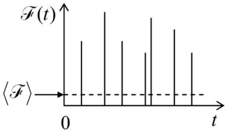
What are the r.m.s. fluctuations of other thermodynamic variables – like \(V\), \(T\), etc.? Again, the answer depends on specific conditions. For example, if the volume \(V\) occupied by a gas is externally fixed (say, by rigid walls), it evidently does not fluctuate at all: \(\delta V = 0\). On the other hand, the volume may fluctuate in the situation when the average pressure is fixed – see, e.g., Figure \(1.4.1\). A formal calculation of these fluctuations, using the approach applied in the last section, is complicated by the fact that it is physically impracticable to fix its conjugate variable, \(P\), i.e. suppress its fluctuations. For example, the force \(\mathscr{F}(t)\) exerted by an ideal classical gas on a container's wall (whose measure the pressure is) is the result of individual, independent hits of the wall by particles (Figure \(\PageIndex{1}\)), with the time scale \(\tau_c \sim r_B/\langle v^2\rangle^{1/2} \sim r_B/(T/m)^{1/2} \sim 10^{-16}\) s, so that its frequency spectrum extends to very high frequencies, virtually impossible to control.

Figure \(\PageIndex{1}\): The force exerted by gas particles on a container's wall, as a function of time (schematically).

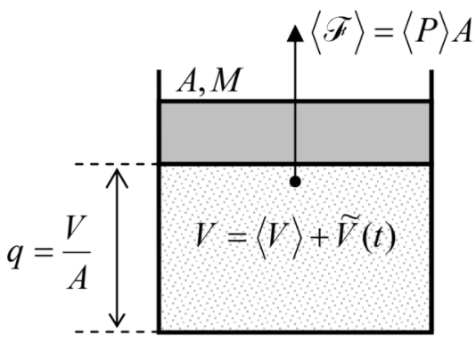
However, we can use the following trick, very typical for the theory of fluctuations. It is almost evident that the r.m.s. fluctuations of the gas volume are independent of the shape of the container. Let us consider a particular situation similar to that shown in Figure \(1.4.1\), with the container of a cylindrical shape, with the base area \(A\).⁸ Then the coordinate of the piston is just \(q = V/A\), while the average force exerted by the gas on the cylinder is \(\mathscr{F} = PA\) – see Figure \(\PageIndex{2}\). Now if the piston is sufficiently massive, its free oscillation frequency \(\omega\) near the equilibrium position is small enough to satisfy the following three conditions.

First, besides balancing the average force \(\langle \mathscr{F} \rangle\) and thus sustaining the average pressure \(\langle P\rangle = \langle \mathscr{F} \rangle /A\) of the gas, the interaction between the heavy piston and the relatively light particles of the gas is weak, because of a relatively short duration of the particle hits (Figure \(\PageIndex{1}\)). As a result, the full energy of the system may be represented as a sum of those of the particles and the piston, with a quadratic contribution to the piston's potential energy by small deviations from the equilibrium:

\[U_p = \frac{\kappa}{2} \tilde{q}^2 , \quad \text{ where } \tilde{q} \equiv q - \langle q \rangle = \frac{\tilde{V}}{A}, \label{34}\]

and \(\kappa\) is the effective spring constant arising from the finite compressibility of the gas.

Figure \(\PageIndex{2}\): Deriving Equation (\ref{37a}-\ref{37b}).

Second, at \(\omega \rightarrow 0\), this spring constant may be calculated just as for constant variations of the volume, with the gas remaining in quasi-equilibrium at all times:

\[\kappa = - \frac{\partial \langle \mathscr{F}\rangle}{\partial q} = A^2 \left( - \frac{\partial \langle P \rangle }{\partial \langle V \rangle } \right). \label{35}\]

This partial derivative⁹ should be calculated at whatever the given thermal conditions are, e.g., with \(S =\) const for adiabatic conditions (i.e., a thermally insulated gas), or with \(T =\) const for isothermal conditions (including a good thermal contact between the gas and a heat bath), etc. With that constant denoted as \(X\), Eqs. (\ref{34})-(\ref{35}) give

\[U_p = \frac{1}{2} \left( - A^2 \frac{\partial \langle P \rangle }{\partial \langle V \rangle }\right)_X \left(\frac{\tilde{V}}{A}\right)^2 \equiv \frac{1}{2} \left(-\frac{\partial \langle P \rangle}{\partial \langle V \rangle}\right)_X \tilde{V}^2. \label{36}\]

Fluctuations of \(V\):

\[\boxed{ \langle \tilde{V}^2 \rangle_X = T \left( - \frac{\partial \langle V \rangle }{\partial \langle P \rangle} \right)_X. } \label{37a}\]

Since this result is valid for any \(A\) and \(\omega \), it should not depend on the system's geometry and piston's mass, provided that it is large in comparison with the effective mass of a single system component (say, a gas molecule) – the condition that is naturally fulfilled in most experiments. For the particular case of fluctuations at constant temperature \((X = T)\),¹¹ we may use the definition (\(3.3.7\)) of the isothermal bulk compressibility \(K_T\) of the gas to rewrite Equation (\ref{37a}) as

\[\langle \tilde{V}^2 \rangle_T = \frac{TV}{K_T}. \label{37b}\]

For an ideal classical gas of \(N\) particles, with the equation of state \(\langle V\rangle = NT/\langle P\rangle \), it is easier to use directly Equation (\ref{37a}), again with \(X = T\), to get

\[\langle \tilde{V}^2 \rangle_T = -T \left( - \frac{NT}{\langle P \rangle^2} \right) = \frac{\langle V \rangle^2}{N}, \quad \text{ i.e. } \frac{\delta V_T}{\langle V \rangle } = \frac{1}{N^{1/2}}, \label{38}\]

in full agreement with the general trend given by Equation (\(5.1.13\)).

Now let us proceed to fluctuations of temperature, for simplicity focusing on the case \(V =\) const. Let us again assume that the system we are considering is weakly coupled to a heat bath of temperature \(T_0\), in the sense that the time \(\tau\) of temperature equilibration between the two is much larger than the time of internal equilibration, called thermalization. Then we may assume that, on the former time scale, \(T\) changes virtually simultaneously in the whole system, and consider it a function of time alone:

\[T = \langle T \rangle + \tilde{T} (t). \label{39}\]

Moreover, due to the (relatively) large \(\tau \), we may use the stationary relation between small fluctuations of temperature and the internal energy of the system:

\[\tilde{T} (t) = \frac{\tilde{E}(t)}{C_V}, \text{ so that } \delta T = \frac{\delta E}{C_V}. \label{40}\]

With those assumptions, Equation (\(5.2.6\)) immediately yields the famous expression for the so-called thermodynamic fluctuations of temperature:

Fluctuations of \(T\):

\[\boxed{\delta T = \frac{\delta E}{C_V} = \frac{\langle T \rangle}{C_V^{1/2}}. } \label{41}\]

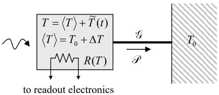
The most straightforward application of this result is to analyses of so-called bolometers – broadband detectors of electromagnetic radiation in microwave and infrared frequency bands. (In particular, they are used for measurements of the CMB radiation, which was discussed in Sec. 2.6). In such a detector (Figure \(\PageIndex{3}\)), the incoming radiation is focused on a small sensor (e.g., either a small piece of a germanium crystal or a superconductor thin film at temperature \(T \approx T_c\), etc.), which is well isolated thermally from the environment. As a result, the absorption of an even small radiation power \(\mathscr{P}\) leads to a noticeable change \(\Delta T\) of the sensor's average temperature \(\langle T\rangle\) and hence of its electric resistance \(R\), which is probed up by low-noise external electronics.¹² If the power does not change in time too fast, \(\Delta T\) is a certain function of \(\mathscr{P}\), turning to 0 at \(\mathscr{P} = 0\). Hence, if \(\Delta T\) is much lower than the environment temperature \(T_0\), we may keep only the main, linear term in its Taylor expansion in \(\mathscr{P}\):

\[ \Delta T \equiv \langle T \rangle −T_0 = \frac{\mathscr{P}}{\mathscr{G}}, \label{42}\]

where the coefficient \(\mathscr{G} \equiv \partial \mathscr{P}/\partial T\) is called the thermal conductance of the (perhaps small but unavoidable) thermal coupling between the sensor and the heat bath – see Figure \(\PageIndex{3}\).

Figure \(\PageIndex{3}\): The conceptual scheme of a bolometer.

The power may be detected if the electric signal from the sensor, which results from the change \(\Delta T\), is not drowned in spontaneous fluctuations. In practical systems, these fluctuations are contributed by several sources including electronic amplifiers. However, in modern systems, these “technical” contributions to noise are successfully suppressed,¹³ and the dominating noise source is the fundamental sensor temperature fluctuations, described by Equation (\ref{41}). In this case, the so-called noise-equivalent power (“NEP”), defined as the level of \(\mathscr{P}\) that produces the signal equal to the r.m.s. value of noise, may be calculated by equating the expressions (\ref{41}) (with \(\langle T\rangle = T_0\)) and (\ref{42}):

\[\text{NEP} \equiv \left. \mathscr{P} \right|_{\Delta T = \delta T} = \frac{T_0 \mathscr{G}}{C_V^{1/2}}. \label{43}\]

This expression shows that to decrease the NEP, i.e. improve the detector's sensitivity, both the environment temperature \(T_0\) and the thermal conductance \(\mathscr{G}\) should be reduced. In modern receivers of radiation, their typical values are of the order of 0.1 K and \(10^{-10}\) W/K, respectively.

On the other hand, Equation (\ref{43}) implies that to increase the bolometer's sensitivity, i.e. to reduce the NEP, the \(C_V\) of the sensor, and hence its mass, should be increased. This conclusion is valid only to a certain extent, because due to technical reasons (parameter drifts and the so-called \(1/f\) noise of the sensor and external electronics), the incoming power has to be modulated with as high frequency \(\omega\) as technically possible (in practical receivers, the cyclic frequency \(\nu = \omega /2\pi\) of the modulation is between 10 and 1,000 Hz), so that the electrical signal might be picked up from the sensor at that frequency. As a result, the \(C_V\) may be increased only until the thermal constant of the sensor,

\[ \tau = \frac{C_V}{\mathscr{G}}, \label{44}\]

becomes close to \(1/\omega \), because at \(\omega \tau >> 1\) the useful signal drops faster than noise. So, the lowest (i.e. the best) values of the NEP,

\[(\text{NEP})_{min} = \alpha T_0 \mathscr{G}^{1/2} v^{1/2}, \quad \text{ with } \alpha \sim 1, \label{45}\]

are reached at \(\nu\tau \approx 1\). (The exact values of the optimal product \(\omega \tau \), and of the numerical constant \(\alpha \sim 1\) in Equation (\ref{45}), depend on the exact law of the power modulation in time, and the readout signal processing procedure.) With the parameters cited above, this estimate yields \((\text{NEP})_{min}/\nu^{1/2} \sim 3 \times 10^{-17} \) W/Hz\(^{1/2}\) – a very low power indeed.

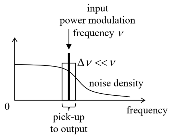
However, perhaps counter-intuitively, the power modulation allows the bolometric (and other broadband) receivers to register radiation with power much lower than this NEP! Indeed, picking up the sensor signal at the modulation frequency \(\omega \), we can use the subsequent electronics stages to filter out all the noise besides its components within a very narrow band, of width \(\Delta \nu << \nu\), around the modulation frequency (Figure \(\PageIndex{4}\)). This is the idea of a microwave radiometer,¹⁴ currently used in all sensitive broadband receivers of radiation.

Figure \(\PageIndex{4}\): The basic idea of the Dicke radiometer.

In order to analyze this opportunity, we need to develop theoretical tools for a quantitative description of the spectral distribution of fluctuations. Another motivation for that description is a need for analysis of variables dominated by fast (high-frequency) components, such as pressure – please have one more look at Figure \(\PageIndex{1}\). Finally, during such an analysis, we will run into the fundamental relation between fluctuations and dissipation, which is one of the main results of statistical physics as a whole.