5.6: The Kramers problem and the Smoluchowski equation

Returning to the classical case, it is evident that Langevin equations of the type (\(5.5.3\)) provide means not only for the analysis of stationary fluctuations, but also for the description of arbitrary time evolution of (classical) systems coupled to their environments – which, again, may provide both dissipation and fluctuations. However, this approach to evolution analysis suffers from two major handicaps.

First, the Langevin equation does enable a straightforward calculation of the statistical average of the variable \(q\), and its fluctuation variance – i.e., in the common mathematical terminology, the first and second moments of the probability density \(w(q, t)\) – as functions of time, but not of the probability distribution as such. Admittedly, this is rarely a big problem, because in most cases the distribution is Gaussian – see, e.g., Equation (\(2.5.12\)).

\[m\ddot{q}+\eta\dot{q} + \frac{\partial U (q,t)}{\partial q} = \tilde{\mathscr{F}}(t), \label{107}\]

valid for an arbitrary, possibly time-dependent potential \(U(q, t)\). Unfortunately, the solution of this equation may be very hard. Indeed, its Fourier analysis carried out in the last section was essentially based on the linear superposition principle, which is invalid for nonlinear equations.

If the fluctuation intensity is low, \(\left| \delta q \right| << \langle q\rangle \), where \(\langle q\rangle (t)\) is the deterministic solution of Equation (\ref{107}) in the absence of fluctuations, this equation may be linearized⁵⁴ with respect to small fluctuations \(\tilde{q} \equiv q − \langle q \rangle \) to get a linear equation,

\[m\ddot{\tilde{q}}+\eta\dot{\tilde{q}}+\kappa (t) \tilde{q} = \tilde{\mathscr{F}}(t), \quad \text{ with } \kappa (t) \equiv \frac{\partial^2}{\partial q^2} U(\langle q \rangle (t),t). \label{108}\]

However, some important problems cannot be solved by linearization. Perhaps, the most apparent (and practically very important) example is the so-called Kramers problem⁵⁶ of finding the lifetime of a metastable state of a 1D classical system in a potential well separated from the region of unlimited motion with a potential barrier – see Figure \(\PageIndex{1}\).

Figure \(\PageIndex{1}\): The Kramers problem.

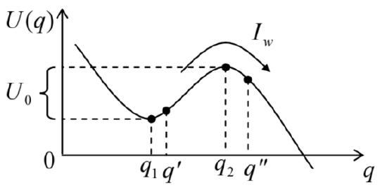
In the absence of fluctuations, the system, initially placed close to the well's bottom (in Figure \(\PageIndex{1}\), at \(q \approx q_1\)), would stay there forever. Fluctuations result not only in a finite spread of the probability density \(w(q, t)\) around that point but also in a gradual decrease of the total probability

\[W(t) = \int_{\text{well's bottom}} w(q,t) dq \label{109}\]

to find the system in the well, because of a non-zero rate of its escape from it, over the potential barrier, due to thermal activation. What may be immediately expected of the situation is that if the barrier height,

\[U_0 \equiv U(q_2) - U(q_1), \label{110}\]

is much larger than temperature \(T\),⁵⁷ the Boltzmann distribution \(w \propto \exp\{-U(q)/T\}\) should be still approximately valid in most of the well, so that the probability for the system to overcome the barrier should scale as \(\exp\{-U_0/T\}\). From these handwaving arguments, one may reasonably expect that if the probability \(W(t)\) of the system's still residing in the well by time \(t\) obeys the usual “decay law”

\[\dot{W} = -\frac{W}{\tau} \label{111a}\]

then the lifetime \(\tau\) has to obey the general Arrhenius law:

\[\tau = \tau_A \exp \left\{\frac{U_0}{T}\right\}. \label{111b}\]

However, these relations need to be proved, and the pre-exponential coefficient \(\tau_A\) (usually called the attempt time) needs to be calculated. This cannot be done by the linearization of Equation (\ref{107}), because this approximation is equivalent to a quadratic approximation of the potential \(U(q)\), which evidently cannot describe the potential well and the potential barrier simultaneously – see Figure \(\PageIndex{1}\) again.

This and other essentially nonlinear problems may be addressed using an alternative approach to fluctuations, dealing directly with the time evolution of the probability density \(w(q, t)\). Due to the shortage of time/space, I will review this approach using mostly handwaving arguments, and refer the interested reader to special literature⁵⁸ for strict mathematical proofs. Let us start from the diffusion of a free classical 1D particle with inertial effects negligible in comparison with damping. It is described by the Langevin equation (\(5.5.13\)) with \(\mathscr{F}_{det} = 0\). Let us assume that at all times the probability distribution stays Gaussian:

\[w(q,t) = \frac{1}{(2\pi)^{1/2} \delta q(t) } \exp \left\{ - \frac{(q - q_0)^2}{2\delta q^2(t)}\right\}, \label{112}\]

where \(q_0\) is the initial position of the particle, and \(\delta q(t)\) is the time-dependent distribution width, whose growth in time is described, as we already know, by Equation (\(5.5.16\)):

\[\delta q (t) = (2Dt)^{1/2} . \label{113}\]

\[\frac{\partial w}{\partial t} = D \frac{\partial^2 w}{\partial q^2}, \label{114}\]

with the delta-functional initial condition

\[w (q,0) = \delta (q - q_0). \label{115}\]

The simple and important equation of diffusion (\ref{114}) may be naturally generalized to the 3D motion:⁶⁰

Equation of diffusion:

\[\boxed{\frac{\partial w}{\partial t} = D \nabla^2 w. } \label{116}\]

\[\frac{\partial w}{\partial t} + \boldsymbol{\nabla} \cdot \mathbf{j}_w = 0, \label{117a}\]

where the vector \(\mathbf{j}_w\) has the physical sense of the probability current density. (The validity of this relation is evident from its integral form,

\[\frac{d}{dt} \int_V wd^3 r + \oint_S \mathbf{j}_w \cdot d^2 \mathbf{q} = 0, \label{117b}\]

which results from the integration of Equation (\ref{117a}) over an arbitrary time-independent volume \(V\) limited by surface \(S\), and applying the divergence theorem⁶² to the second term.) The continuity relation (\ref{117a}) coincides with Equation (\ref{116}), with \(D\) given by Equation (\(5.5.17\)), only if we take

\[\mathbf{j}_w = -D \boldsymbol{\nabla} w = - \frac{T}{\eta} \boldsymbol{\nabla} w . \label{118}\]

The first form of this relation allows a simple interpretation: the probability flow is proportional to the spatial gradient of the probability density (i.e., in application to \(N >> 1\) similar and independent particles, just to the gradient of their concentration \(n = Nw\)), with the sign corresponding to the flow from the higher to lower concentrations. This flow is the very essence of the effect of diffusion. The second form of Equation (\ref{118}) is also not very surprising: the diffusion speed scales as temperature and is inversely proportional to the viscous drag.

The fundamental Equation (\ref{117a}-\ref{117b}) has to be satisfied also in the case of a force-driven particle at negligible diffusion (\(D \rightarrow 0\)); in this case

\[\mathbf{j}_w = w\mathbf{v} , \label{119}\]

where \(\mathbf{v}\) is the deterministic velocity of the particle. In the high-damping limit we are considering right now, \(\mathbf{v}\) has to be just the drift velocity:

\[\mathbf{v} = \frac{1}{\eta} \pmb{\mathscr{F}}_{det} = - \frac{1}{\eta} \boldsymbol{\nabla} U(\mathbf{q}), \label{120}\]

where \(\pmb{\mathscr{F}}_{det}\) is the deterministic force described by the potential energy \(U(\mathbf{q})\).

Now that we have descriptions of \(\mathbf{j}_w\) due to both the drift and the diffusion separately, we may rationally assume that in the general case when both effects are present, the corresponding components (\ref{118}) and (\ref{119}) of the probability current just add up, so that

\[\mathbf{j}_w = \frac{1}{\eta} [w (- \boldsymbol{\nabla} U) - T \boldsymbol{\nabla} w ], \label{121}\]

and Equation (\ref{117a}) takes the form

Smoluchowski equation:

\[\boxed{ \eta \frac{\partial w}{\partial t} = \boldsymbol{\nabla} ( w \boldsymbol{\nabla} U ) + T \nabla^2 w. } \label{122}\]

This is the Smoluchowski equation,⁶³ which is closely related to the drift-diffusion equation in multi particle kinetics – to be discussed in the next chapter.

As a sanity check, let us see what the Smoluchowski equation gives in the stationary limit, \(\partial w/\partial t \rightarrow 0\) (which evidently may be eventually achieved only if the deterministic potential \(U\) is time independent.) Then Equation (\ref{117a}) yields \(\mathbf{j}_w =\) const, where the constant describes the deterministic motion of the system as the whole. If such a motion is absent, \(\mathbf{j}_w = 0\), then according to Equation (\ref{121}),

\[w\boldsymbol{\nabla} U + T \boldsymbol{\nabla} w = 0, \quad \text{ i.e. } \frac{\boldsymbol{\nabla} w}{w} = -\frac{\boldsymbol{\nabla}U}{T}. \label{123}\]

Since the left-hand side of the last relation is just \(\boldsymbol{\nabla} (\ln w)\), it may be easily integrated over \(\mathbf{q}\), giving

\[\ln w = - \frac{U}{T} + \ln C , \quad \text{ i.e. } w(\mathbf{r}) = C \exp \left\{ - \frac{U(\mathbf{q})}{T} \right\}, \label{124}\]

where \(C\) is a normalization constant. With both sides multiplied by the number \(N\) of similar, independent systems, with the spatial density \(n(\mathbf{q}) = Nw(\mathbf{q})\), this equality becomes the Boltzmann distribution (\(3.1.28\)).

As a less trivial example of the Smoluchowski equation's applications, let us use it to solve the 1D Kramers problem (Figure \(\PageIndex{1}\)) in the corresponding high-damping limit, \(m << \eta \tau_A\), where \(\tau_A\) (still to be calculated) is some time scale of the particle's motion inside the well. It is straightforward to verify that the 1D version of Equation (\ref{121}),

\[I_w = \frac{1}{\eta} \left[ w \left( - \frac{\partial U}{\partial q}\right) - T \frac{\partial w}{\partial q} \right], \label{125a}\]

(where \(I_w\) is the probability current at a certain point \(q\), rather than its density) is mathematically equivalent to

\[I_w = - \frac{T}{\eta} \exp \left\{ - \frac{U(q)}{T} \right\} \frac{\partial}{\partial q} \left( w \exp \left\{ \frac{U(q)}{T}\right\}\right), \label{125b}\]

so that we may write

\[I_w \exp \left\{ \frac{U(q)}{T} \right\} = - \frac{T}{\eta} \frac{\partial}{\partial q} \left( w \exp \left\{ \frac{U(q)}{T}\right\}\right). \label{126}\]

As was discussed above, the notion of metastable state's lifetime is well defined only for sufficiently low temperatures

\[ T << U_0 . \label{127}\]

when the lifetime is relatively long: \(\tau >> \tau_A\). Since according to Equation (\ref{111a}), the first term of the continuity equation (\ref{117b}) has to be of the order of \(W/\tau \), in this limit the term, and hence the gradient of \(I_w\), are exponentially small, so the probability current virtually does not depend on \(q\) in the potential barrier region. Let us use this fact at the integration of both sides of Equation (\ref{126}) over that region:

\[I_w \int^{q^{\prime\prime}}_{q'} \exp \left\{ \frac{U(q)}{T} \right\} dq = -\frac{T}{\eta} \left( w \exp \left\{ \frac{U(q)}{T}\right\}\right)^{q^{\prime\prime}}_{q'}, \label{128}\]

where the integration limits \(q'\) and \(q^{\prime\prime}\) (see Figure \(\PageIndex{1}\)) are selected so that

\[T << U(q') −U(q_1 ),U(q_2 ) −U(q^{\prime\prime}) << U_0 . \label{129}\]

(Obviously, such selection is only possible if the condition (\ref{127}) is satisfied.) In this limit, the contribution from the point \(q^{\prime\prime}\) to the right-hand side of Equation (\ref{129}) is negligible because the probability density behind the barrier is exponentially small. On the other hand, the probability at the point \(q'\) has to be close to the value given by its quasi-stationary Boltzmann distribution (\ref{124}), so that

\[w(q') \exp \left\{ \frac{U(q')}{T} \right\} = w(q_1) \exp \left\{ \frac{U(q_1)}{T}\right\}, \label{130}\]

and Equation (\ref{128}) yields

\[I_w = \frac{T}{\eta} w(q_1) / \int^{q^{\prime\prime}}_{q'} \exp \left\{ \frac{U(q) - U(q_1)}{T} \right\} dq. \label{131}\]

Patience, my reader, we are almost done. The probability density \(w(q_1)\) at the well's bottom may be expressed in terms of the total probability \(W\) of the particle being in the well by using the normalization condition

\[W = \int_{\text{well's bottom}} w(q_1) \exp \left\{ \frac{U(q_1) - U(q)}{T} \right\} dq; \label{132}\]

the integration here may be limited to the region where the difference \(U(q) – U(q_1)\) is much smaller than \(U_0\) – cf. Equation (\ref{129}). According to the Taylor expansion, the shape of virtually any smooth potential \(U(q)\) near the point \(q_1\) of its minimum may be well approximated with a quadratic parabola:

\[U\left(q \approx q_{1}\right)-U\left(q_{1}\right) \approx \frac{\kappa_1}{2} \left(q-q_{1}\right)^{2} \quad \text { where } \kappa_{1} \equiv-\left.\frac{d^{2} U}{d q^{2}}\right|_{q=q_{1}}>0. \label{133}\]

\[W = w(q_1) \int_{\text{well's bottom}} \exp \left\{ - \frac{ \kappa_1 (q-q_1)^2}{2T} \right\} dq \approx w(q_1) \int^{+\infty}_{-\infty} \exp \left\{\frac{\kappa_1 \tilde{q}^2}{2T}\right\} d\tilde{q} = w(q_1)\left(\frac{2\pi T}{\kappa_1}\right)^{1/2}. \label{134}\]

To complete the calculation, we may use a similar approximation for the barrier top:

\[U\left(q \approx q_{2}\right)-U\left(q_{1}\right) \approx\left[U\left(q_{2}\right)-\frac{\kappa_{2}}{2}\left(q-q_{2}\right)^{2}\right]-U\left(q_{1}\right)=U_{0}-\frac{\kappa_{2}}{2}\left(q-q_{2}\right)^{2} \\
\text { where } \kappa_{2} \equiv-\left.\frac{d^{2} U}{d q^{2}}\right|_{q=q_{2}}>0, \label{135}\]

and work out the remaining integral in Equation (\ref{131}), because in the limit (\ref{129}) it is dominated by the contribution from a region very close to the barrier top, where the approximation (\ref{135}) is asymptotically exact. As a result, we get

\[\int^{q^{\prime\prime}}_{q'} \exp \left\{\frac{U(q)-U(q_1)}{T}\right\} dq \approx \exp \left\{\frac{U_0}{T}\right\} \left(\frac{2\pi T}{\kappa_2}\right)^{1/2}. \label{136}\]

Plugging Equation (\ref{136}), and the \(w(q_1)\) expressed from Equation (134), into Equation (\ref{131}), we finally get

\[I_w = W \frac{(\kappa_1\kappa_2)^{1/2}}{2\pi \eta} \exp \left\{-\frac{U_0}{T}\right\}. \label{137}\]

This expression should be compared with the 1D version of Equation (\ref{117b}) for the segment \([–\infty , q']\). Since this interval covers the region near \(q_1\) where most of the probability density resides, and \(I_q(-\infty ) = 0\), this equation is merely

\[\frac{dW}{dt} + I_w (q') = 0. \label{138}\]

In our approximation, \(I_w(q')\) does not depend on the exact position of the point \(q'\), and is given by Equation (\ref{137}), so that plugging it into Equation (\ref{138}), we recover the exponential decay law (\ref{111a}), with the lifetime \(\tau\) obeying the Arrhenius law (\ref{111b}), and the following attempt time:

Kramers formula for high damping:

\[\boxed{ \tau_A = \frac{2\pi \eta}{(\kappa_1\kappa_2 )^{1/2}} \equiv 2\pi (\tau_1 \tau_2 )^{1/2} , \text{ where } \tau_{1,2} \equiv \frac{\eta}{\kappa_{1,2}}.} \label{139}\]

Thus the metastable state lifetime is indeed described by the Arrhenius law, with the attempt time scaling as the geometric mean of the system's “relaxation times” near the potential well bottom \((\tau_1)\) and the potential barrier top \((\tau_2)\).⁶⁵ Let me leave for the reader's exercise to prove that if the potential profile near well's bottom and/or top is sharp, the expression for the attempt time should be modified, but the Arrhenius decay law (\ref{111a}-\ref{111b}) is not affected.