
5.7: The Fokker-Planck Equation


- Last updated
- Sep 20, 2022
- Save as PDF

( \newcommand{\kernel}{\mathrm{null}\,}\)
Formula (5.6.36) is just a particular, high-damping limit of a more general result obtained by Kramers. In order to get all of it (and much more), we need to generalize the Smoluchowski equation to arbitrary values of damping η. In this case, the probability density w is a function of not only the particle's position q (and time t) but also of its momentum p – see Equation (2.1.11). Thus the continuity equation (5.6.12−6.6.13) needs to be generalized to the 6D phase space {q,p}. Such generalization is natural:
∂w∂t+∇q⋅jq+∇p⋅jp=0,
where jq (which was called jw in the last section) is the probability current density in the coordinate space, and ∇q (which was denoted as ∇ in that section) is the usual vector operator in the space, while jp is the current density in the momentum space, and ∇p is the similar vector operator in that space:
∇q≡3∑j=1nj∂∂qj,∇p≡3∑j=1nj∂∂pj.
At negligible fluctuations (T→0), jp may be composed using the natural analogy with jq – see Equation (5.6.15). In our new notation, that relation reads,
jq=w˙q=wpm
so it is natural to take
jp=w˙p=w⟨FF⟩,
where the (statistical-ensemble) averaged force ⟨FF⟩ includes not only the contribution due to the potential's gradient, but also the drag force –ηv provided by the environment – see Equation (5.5.2) and its discussion:
jp=w(−∇qU−ηv=−w(∇qU+ηpm).
As a sanity check, it is straightforward to verify that the diffusion-free equation resulting from the combination of Eqs. (???), (???) and (???-???),
∂w∂t|drift=−∇q⋅(wpw)+∇p⋅[w(∇qU+ηpm)],
allows the following particular solution:
w(q,p,t)=δ[q−q(t)]δ[p−⟨p⟩(t)],
where the statistical-averaged coordinate and momentum satisfy the deterministic equations of motion,
⟨˙q⟩=⟨p⟩m,⟨˙p⟩=−∇qU−η⟨p⟩m,
describing the particle's drift, with the usual deterministic initial conditions.
In order to understand how the diffusion should be accounted for, let us consider a statistical ensemble of free (∇qU=0,η→0) particles that are uniformly distributed in the direct space q (so that ∇qw=0), but possibly localized in the momentum space. For this case, the right-hand side of Equation (???) vanishes, i.e. the time evolution of the probability density w may be only due to diffusion. In the corresponding limit ⟨FF⟩→0, the Langevin equation (5.6.1) for each Cartesian coordinate is reduced to
m¨qj=˜Fj(t), i.e. ˙pj=˜Fj(t).
The last equation is identical to the high-damping 1D equation (5.5.3) (with Fdet=0), with the replacement q→pj/η, and hence the corresponding contribution to ∂w/∂t may be described by the last term of Equation (5.6.18), with that replacement:
∂w∂t|diffusion=D∇2p/ηw=Tηη2∇2pw≡ηT∇2pw.
Now the reasonable assumption that in the arbitrary case the drift and diffusion contributions to ∂w/∂t just add up immediately leads us to the full Fokker-Planck equation:66
Fokker-Planck equation:
∂w∂t=−∇q⋅(wpm)+∇p⋅[w(∇qU+ηpm)]+ηT∇2pw.
As a sanity check, let us use this equation to calculate the stationary probability distribution of the momentum of particles with an arbitrary damping η but otherwise free, in the momentum space, assuming (just for simplicity) their uniform distribution in the direct space, ∇q=0. In this case, Equation (???) is reduced to
∇p⋅[w(ηpm)]+ηT∇2pw=0, i.e ∇p⋅(pmw+T∇pw)=0.
The first integration over the momentum space yields
pmw+T∇pw=jw, i.e. w∇p(p22m)+T∇pw=jw,
where jw is a vector constant describing a possible general probability flow in the system. In the absence of such flow, jw=0, we get
∇p(p22m)+T∇pww≡∇p(p22m+Tlnw)=0, giving w=const×exp{−p22mT},
i.e. the Maxwell distribution (3.1.5). However, the result (???) is more general than that obtained in Sec. 3.1, because it shows that the distribution stays the same even at non-zero damping. It is easy to verify that in the more general case of an arbitrary stationary potential U(q), Equation (???) is satisfied with the stationary solution (3.1.25), also giving jw=0.
It is also straightforward to show that if the damping is large (in the sense assumed in the last section), the solution of the Fokker-Planck equation tends to the following product
w(q,p,t)→const×exp{−p22mT}×w(q,t),
where the direct-space distribution w(q,t) obeys the Smoluchowski equation (5.6.18).
Another important particular case is that of a quasi-periodic motion of a particle, with low damping, in a soft potential well. In this case, the Fokker-Planck equation describes both diffusion of the effective phase Θ of such (generally nonlinear, “anharmonic”) oscillator, and slow relaxation of its energy. If we are only interested in the latter process, Equation (???) may be reduced to the so-called energy diffusion equation,67 which is easier to solve.
However, in most practically interesting cases, solutions of Equation (???) are rather complicated. (Indeed, the reader should remember that these solutions embody, in the particular case T=0, all classical dynamics of a particle.) Because of this, I will present (rather than derive) only one more of them: the solution of the Kramers problem (Figure 5.6.1). Acting almost exactly as in Sec. 6, one can show68 that at virtually arbitrary damping (but still in the limit T<<U0), the metastable state's lifetime is again given by the Arrhenius formula (5.6.6), with the attempt time again expressed by the first of Eqs. (5.6.36), but with the reciprocal time constants 1/τ1,2 replaced with
ω1,2≡[ω21,2+(η2m)2]1,2−η2m→{ω1,2for η<<mω1,2,1/τ1,2,for mω1,2<<η,
where ω1,2≡(κ1,2/m)1/2, and κ1,2 are the effective spring constants defined by Eqs. (5.6.30) and (5.6.32). Thus, in the important particular limit of low damping, Eqs. (5.6.6) and (???) give the famous formula
Kramers formula for low damping:
τ=2π(ω1ω2)1/2exp{U0T}.
This Kramers' result for the classical thermal activation of the dissipation-free system over a potential barrier may be compared with that for its quantum-mechanical tunneling through the barrier.69 The WKB approximation for the latter effect gives the expression
τQ=τAexp{−2∫κ2(q)>0κ(q)dq}, with ℏ2κ2(q)2m≡U(q)−E,
showing that generally, the classical and quantum lifetimes of a metastable state have different dependences on the barrier shape. For example, for a nearly-rectangular potential barrier, the exponent that determines the classical lifetime (???) depends (linearly) only on the barrier height U0, while that defining the quantum lifetime (???) is proportional to the barrier width and to the square root of U0. However, in the important case of “soft” potential profiles, which are typical for the case of barely emerging (or nearly disappearing) quantum wells (Figure 5.7.1), the classical and quantum results are closely related.
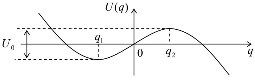
U(q)=aq−b3q3.
(For the particle's escape into the positive direction of the q-axis, we should have a,b>0.) An easy calculation gives all essential parameters of this cubic parabola: the positions of its minimum and maximum:
q2=−q1=(a/b)1/2,
the barrier height over the well's bottom:
U0≡U(q2)−U(q1)=43(a3b)1/2,
and the effective spring constants at these points:
κ1=κ2≡|d2Udq2|q1,2=2(ab)1/2.
The last expression shows that for this potential profile, the frequencies ω1,2 participating in Equation (???) are equal to each other, so that this result may be rewritten as
Soft well: thermal lifetime
τ=2πω0exp{U0T}, with ω20≡2(ab)1/2m.
On the other hand, for the same profile, the WKB approximation (???) (which is accurate when the height of the metastable state energy over the well's bottom, E–U(q1)≈ℏω0/2, is much lower than the barrier height U0) yields71
Soft well: quantum lifetime
τQ=2πω0(ℏω0864U0)1/2exp{365U0ℏω0}.
The comparison of the dominating, exponential factors in these two results shows that the thermal activation yields a lower lifetime (i.e., dominates the metastable state decay) if the temperature is above the crossover value
Tc=365ℏω≡7.2ℏω.
This expression for the cubic-parabolic barrier may be compared with the similar crossover for a quadratic-parabolic barrier,72 for which Tc=2πℏω0≈6.28ℏω0. We see that the numerical factors for the quantum-to-classical crossover temperature for these two different soft potential profiles are close to each other – and much larger than 1, which could result from a naïve estimate.