5.8: Back to the correlation function

Unfortunately, I will not have time/space to either derive or even review solutions of other problems using the Smoluchowski and Fokker-Planck equations, but have to mention one conceptual issue. Since it is intuitively clear that the solution \(w(\mathbf{q}, \mathbf{p}, t)\) of the Fokker-Planck equation for a system provides the complete statistical information about it, one may wonder how it may be used to find its temporal characteristics that were discussed in Secs. 4-5, using the Langevin formalism. For any statistical average of a function taken at the same time instant, the answer is clear – cf. Equation (\(2.1.11\)):

\[\langle f[ \mathbf{q}(t), \mathbf{p}(t)] \rangle = \int f(\mathbf{q},\mathbf{p}) w (\mathbf{q}, \mathbf{p}, t) d^3 qd^3 p, \label{164}\]

but what if the function depends on variables taken at different times, for example as in the correlation function \(K_f(\tau )\) defined by Equation (\(5.4.3\))?

To answer this question, let us start from the discrete-variable case when Equation (\ref{164}) takes the form (\(2.1.7\)), which, for our current purposes, may be rewritten as

\[\langle f(t)\rangle = \sum_m f_m W_m (t). \label{165}\]

In plain English, this is a sum of all possible values of the function, each multiplied by its probability as a function of time. But this implies that the average \(\langle f(t)f(t')\rangle\) may be calculated as the sum of all possible products \(f_mf_{m'}\), multiplied by the joint probability to measure outcome \(m\) at moment \(t\), and outcome \(m'\) at moment \(t'\). The joint probability may be represented as a product of \(W_m(t)\) by the conditional probability \(W(m', t'| m, t)\). Since the correlation function is well defined only for stationary systems, in the last expression we may take \(t = 0\), i.e. look for the conditional probability as the solution, \(W_{m'}(\tau )\), of the equation describing the system's probability evolution, at time \(\tau = t' – t\) (rather than \(t'\)), with the special initial condition

\[ W_{m'}(0) = \delta_{ m',m }. \label{166}\]

On the other hand, since the average \(\langle f(t)f(t +\tau )\rangle\) of a stationary process should not depend on \(t\), instead of \(W_m(0)\) we may take the stationary probability distribution \(W_m(\infty )\), independent of the initial conditions, which may be found as the same special solution, but at time \(\tau \rightarrow \infty \). As a result, we get

Correlation function: discrete system

\[\boxed{ \langle f(t) f (t + \tau ) \rangle = \sum_{ m,m'} f_m W_m (\infty ) f_{m'} W_{m'} (\tau ). } \label{167}\]

This expression looks simple, but note that this recipe requires solving the time evolution equations for each \(W_{m'}(\tau )\) for all possible initial conditions (\ref{166}). To see how this recipe works in practice, let us revisit the simplest two-level system (see, e.g., Figure \(4.5.4\), which is reproduced in Figure \(\PageIndex{1}\) below in a notation more convenient for our current purposes), and calculate the correlation function of its energy fluctuations.

Figure \(\PageIndex{1}\): Dynamics of a two-level system.

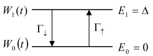
The stationary probabilities of the system's states (i.e. their probabilities for \(\tau \rightarrow \infty \)) have been calculated in problems of Chapter 2, and then again in Sec. 4.4 – see Equation (\(4.4.10\)). In our current notation (Figure \(\PageIndex{1}\)),

\[ W_0 (\infty ) = \frac{1}{1+e^{-\Delta /T}}, \quad W_1 (\infty ) = \frac{1}{e^{\Delta /T} +1}, \\ \text{ so that } \langle E(\infty ) \rangle = W_0 (\infty ) \times 0 + W_1(\infty ) \times \Delta = \frac{\Delta}{e^{\Delta / T}+1}. \label{168}\]

To calculate the conditional probabilities \(W_{m'}(\tau )\) with the initial conditions (\ref{167}) (according to Equation (\ref{168}), we need all four of them, for \(\{m, m'\} = \{0, 1\}\)), we may use the master equations (\(4.5.24\)), in our current notation reading

\[\frac{dW_1}{d\tau} = -\frac{dW_0}{d\tau} = \Gamma_{\uparrow} W_0 - \Gamma_{\downarrow} W_1. \label{169}\]

Since Equation (\ref{169}) conserves the total probability, \(W_0 + W_1 = 1\), only one probability (say, \(W_1\)) is an independent variable, and for it, Equation (\ref{169}) gives a simple, linear differential equation

\[\frac{dW_1}{d\tau} = \Gamma_{\uparrow} - \Gamma_{\Sigma} W_1, \quad \text{ where } \Gamma_{\Sigma} \equiv \Gamma_{\uparrow} + \Gamma_{\downarrow}, \label{170}\]

which may be readily integrated for an arbitrary initial condition:

\[W_1(\tau ) = W_1 (0) e^{-\Gamma_{\Sigma} \tau} + W_1(\infty ) \left(1-e^{-\Gamma_{\Sigma} \tau} \right), \label{171}\]

where \(W_1(\infty )\) is given by the second of Eqs. (\ref{168}). (It is straightforward to verify that the solution for \(W_0(\tau )\) may be represented in a similar form, with the corresponding change of the state index.)

Now everything is ready to calculate the average \(\langle E(t)E(t +\tau )\rangle\) using Equation (\ref{167}), with \(f_{m,m'} = E_{0,1}\). Thanks to our (smart :-) choice of the energy reference, of the four terms in the double sum (\ref{167}), all three terms that include at least one factor \(E_0 = 0\) vanish, and we have only one term left to calculate:

\[\langle E(t) E(t+\tau)\rangle=\left.E_{1} W_{1}(\infty) E_{1} W_{1}(\tau)\right|_{W_{1}(0)=1}=E_{1}^{2} W_{1}(\infty)\left[W_{1}(0) e^{-\Gamma_{\Sigma} \tau}+W_{1}(\infty)\left(1-e^{-\Gamma_{\Sigma} \tau}\right)\right]_{W_{1}(0)=1}\\
=\frac{\Delta^{2}}{e^{\Delta / T}+1}\left[e^{-\Gamma_{\Sigma} \tau}+\frac{1}{e^{\Delta / T}+1}\left(1-e^{-\Gamma_{2} \tau }\right)\right] \equiv \frac{\Delta^{2}}{\left(e^{\Delta / T}+1\right)^{2}}\left(1+e^{\Delta / T} e^{-\Gamma_{\Sigma} \tau}\right) . \label{172}\]

\[K_{E}(\tau) \equiv \langle \tilde{E}(t)\tilde{E}(t+\tau ) \rangle = \langle ( E(t) - \langle E(t) \rangle ) (E(t+\tau ) - \langle E(t)\rangle ) \rangle \\ = \langle E(t) E(t+\tau)\rangle - \langle E(\infty)\rangle^2 = \Delta^2 \frac{e^{\Delta /T}}{\left( E^{\Delta / T} + 1 \right)^2} e^{-\Gamma_{\Sigma} \tau} , \label{173}\]

so that its variance, equal to \(K_E(0)\), does not depend on the transition rates \(\Gamma_{\uparrow}\) and \(\Gamma_{\downarrow}\). However, since the rates have to obey the detailed balance relation (\(4.5.27\)), \(\Gamma_{\downarrow}/\Gamma_{\uparrow} = \exp\{\Delta /T\}\), for this variance we may formally write

\[\frac{K_E (0)}{\Delta^2} = \frac{e^{\Delta / T}}{(e^{\Delta / T} + 1)^2} = \frac{\Gamma_{\downarrow} / \Gamma_{\uparrow}}{(\Gamma_{\downarrow}/\Gamma_{\uparrow} + 1)^2} \equiv \frac{\Gamma_{\uparrow}\Gamma_{\downarrow}}{(\Gamma_{\uparrow} + \Gamma_{\downarrow})^2} \equiv \frac{\Gamma_{\uparrow}\Gamma_{\downarrow}}{\Gamma_{\Sigma}^2}, \label{174}\]

so that Equation (\ref{173}) may be represented in a simpler form:

Energy fluctuations: two-level system

\[\boxed{K_E(\tau ) = \Delta^2 \frac{\Gamma_{\uparrow}\Gamma_{\downarrow}}{\Gamma_{\Sigma}^2} e^{-\Gamma_{\Sigma}\tau}.} \label{175}\]

We see that the correlation function of energy fluctuations decays exponentially with time, with the net rate \(\Gamma_{\Sigma}\). Now using the Wiener-Khinchin theorem (\(5.4.13\)) to calculate its spectral density, we get

\[\boxed{S_E (\omega ) = \frac{1}{\pi} \int^{\infty}_0 \Delta^2 \frac{\Gamma_{\uparrow}\Gamma_{\downarrow}}{\Gamma^2_{\Sigma}} e^{-\Gamma_{\Sigma}\tau} \cos \omega \tau d \tau = \frac{\Delta^2}{\pi\Gamma_{\Sigma}} \frac{\Gamma_{\uparrow}\Gamma_{\downarrow}}{\Gamma^2_{\Sigma} + \omega^2}. } \label{176}\]

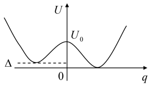
Such Lorentzian dependence on frequency is very typical for discrete-state systems described by master equations. It is interesting that the most widely accepted explanation of the \(1/f\) noise (also called the “flicker” or “excess” noise), which was mentioned in Sec. 5, is that it is a result of thermally activated jumps between states of two-level systems with an exponentially-broad statistical distribution of the transition rates \(\Gamma_{\uparrow\downarrow}\). Such a broad distribution follows from the Kramers formula (\(5.7.17\)), which is approximately valid for the lifetimes of both states of systems with double-well potential profiles (Figure \(\PageIndex{2}\)), for a statistical ensemble with a smooth statistical distribution of the energy barrier heights \(U_0\). Such profiles are typical, in particular, for electrons in disordered (amorphous) solid-state materials, which indeed feature high \(1/f\) noise.

Figure \(\PageIndex{2}\): Typical double-well potential profile.

Returning to the Fokker-Planck equation, we may use the following evident generalization of Equation (\ref{167}) to the continuous-variable case:

Correlation function: continuous system

\[\boxed{ \langle f(t) f(t+\tau) \rangle = \int d^3 q d^3 p \int d^3 q' d^3 p' f(\mathbf{q},\mathbf{p}) w (\mathbf{q},\mathbf{p},\infty ) f(\mathbf{q}', \mathbf{p}' ) w (\mathbf{q}',\mathbf{p}',\tau), } \label{177}\]

were both probability densities are particular values of the equation's solution with the delta-functional initial condition

\[ w(\mathbf{q}',\mathbf{p}',0) = \delta (\mathbf{q}' - \mathbf{q})\delta (\mathbf{p}' - \mathbf{p}). \label{178}\]

For the Smoluchowski equation valid in the high-damping limit, the expressions are similar, albeit with a lower dimensionality:

\[\langle f(t) f(t+\tau)\rangle = \int d^3 q \int d^3 q' f(\mathbf{q})w(\mathbf{q},\infty) f (\mathbf{q}') w (\mathbf{q}',\tau ), \label{179}\]

\[w(\mathbf{q}',0) = \delta (\mathbf{q}'-\mathbf{q}). \label{180}\]

To see this formalism in action, let us use it to calculate the correlation function \(K_q(\tau )\) of a linear relaxator, i.e. an overdamped 1D harmonic oscillator with \(m\omega_0 << \eta \). In this limit, as Equation (\(5.5.3\)) shows, the oscillator's coordinate, averaged over the ensemble of environments, obeys a linear equation,

\[ \eta \langle \dot{q} \rangle + \kappa \langle q \rangle = 0 , \label{181}\]

which describes its exponential relaxation from the initial position \(q_0\) to the equilibrium position \(q = 0\), with the reciprocal time constant \(\Gamma = \kappa /\eta \):

\[\langle q \rangle (t) = q_0 e^{-\Gamma t}. \label{182}\]

The deterministic equation (\ref{181}) corresponds to the quadratic potential energy \(U(q) = \kappa q^2/2\), so that the 1D version of the corresponding Smoluchowski equation (\(5.6.18\)) takes the form

\[\eta \frac{\partial w}{\partial t} = \kappa \frac{\partial}{\partial q} (w q ) + T \frac{\partial^2 w}{\partial q^2}.\label{183}\]

It is straightforward to check, by substitution, that this equation, rewritten for the function \(w(q',\tau )\), with the 1D version of the delta-functional initial condition (\ref{180}), \(w(q',0) = \delta (q' – q)\), is satisfied with a Gaussian function:

\[w(q',\tau) = \frac{1}{(2\pi)^{1/2} \delta q(\tau )} \exp \left\{-\frac{(q'-\langle q \rangle (\tau ) )^2 }{2\delta q^2 (\tau ) } \right\}, \label{184}\]

with its center \(\langle q\rangle (\tau )\) moving in accordance with Equation (\ref{182}), and a time-dependent

\[\delta q^2 (\tau) = \delta q^2 (\infty)(1- e^{2\Gamma \tau}), \quad \text{ where } \delta q^2 (\infty) = \langle q^2 \rangle = \frac{T}{\kappa}. \label{185}\]

(As a sanity check, the last equality coincides with the equipartition theorem's result.) Finally, the first probability under the integral in Equation (\ref{179}) may be found from Equation (\ref{184}) in the limit \(\tau \rightarrow \infty\) (in which \(\langle q\rangle (\tau ) \rightarrow 0\)), by replacing \(q'\) with \(q\):

\[w(q,\infty ) = \frac{1}{(2\pi )^{1/2} \delta q(\infty )} \exp \left\{-\frac{q^2}{2\delta q^2 (\infty ) } \right\}. \label{186}\]

Now all ingredients of the recipe (\ref{179}) are ready, and we can spell it out, for \(f (q) = q\), as

\[\langle q(t) q(t + \tau)\rangle = \frac{1}{2\pi \delta q(\tau ) \delta q (\infty ) } \int^{+\infty}_{-\infty} dq \int^{+\infty}_{-\infty} dq' q \exp \left\{ - \frac{q^2}{2\delta q^2 (\infty ) } \right\} q' \exp \left\{-\frac{(q'-qe^{-\Gamma \tau})^2}{2\delta q^2 (\tau )} \right\}. \label{187}\]

The integral over \(q'\) may be worked our first, by replacing this integration variable with (\(q^{\prime\prime} + qe^{-\Gamma \tau })\) and hence \(dq'\) with \(dq^{\prime\prime}\):

\[\langle q(t) q(t + \tau)\rangle = \frac{1}{2\pi \delta q(\tau ) \delta q (\infty ) } \int^{+\infty}_{-\infty} q \exp \left\{ - \frac{q^2}{2\delta q^2 (\infty ) } \right\} dq \int^{+\infty}_{-\infty} \left(q^{\prime\prime} + qe^{-\Gamma \tau}\right) \exp \left\{-\frac{q^{\prime\prime 2}}{2\delta q^2 (\tau )} \right\} dq^{\prime\prime}. \label{188}\]

The internal integral of the first term in the parentheses equals zero (as that of an odd function in symmetric integration limits), while that with the second term is the standard Gaussian integral, so that

\[\langle q(t) q(t + \tau)\rangle = \frac{1}{(2\pi)^{1/2} \delta q (\infty ) } e^{-\Gamma \tau} \int^{+\infty}_{-\infty} q^2 \exp \left\{ - \frac{q^2}{2\delta q^2 (\infty ) } \right\} dq \equiv \frac{2T}{\pi^{1/2} \kappa} e^{-\Gamma \tau} \int^{+\infty}_{-\infty} \xi^2 \exp \left\{-\xi^2 \right\} d\xi . \label{189}\]

The last integral⁷⁴ equals \(\pi^{1/2}/2\), so that taking into account that for this stationary system centered at the coordinate origin, \(\langle q(\infty )\rangle = 0\), we finally get a very simple result,

Correlation function: linear relaxator

\[\boxed{ K_q (\tau ) \equiv \langle \tilde{q}(t)\tilde{q}(t+\tau)\rangle = \langle q(t)q(t+\tau ) \rangle - \langle q (\infty ) \rangle^2 = \langle q(t) q(t+\tau ) \rangle = \frac{T}{\kappa} e^{-\Gamma \tau}. } \label{190}\]

As a sanity check, for \(\tau = 0\) it yields \(K_q(0) \equiv \langle q^2\rangle = T/\kappa \), in accordance with Equation (\ref{185}). As \(\tau\) is increased the correlation function decreases monotonically – see the solid-line sketch in Figure \(5.4.1\).

\[K_q (\tau ) = 2 \int^{\infty}_0 S_q (\omega ) \cos \omega \tau d \omega = 2 \int^{\infty}_0 \frac{\eta T}{\pi} \frac{1}{\kappa^2 + ( \eta \omega )^2} \cos \omega \tau d\omega \equiv 2\frac{T \Gamma}{\pi} \int^{\infty}_0 \frac{\cos \xi}{(\Gamma \tau )^2 + \xi^2} d\xi = \frac{T}{\kappa} e^{-\Gamma \tau}. \label{191}\]

This example illustrates the fact that for linear systems (and small fluctuations in nonlinear systems) the Langevin approach is usually much simpler than the one based on the Fokker-Planck or Smoluchowski equations. However, again, the latter approach is indispensable for the analysis of fluctuations of arbitrary intensity in nonlinear systems.

To conclude this chapter, I have to emphasize again that the Fokker-Planck and Smoluchowski equations give a quantitative description of the time evolution of nonlinear Brownian systems with dissipation in the classical limit. The description of the corresponding properties of such dissipative (“open”) and nonlinear quantum systems is more complex,⁷⁶ and only a few simple problems of their theory have been solved analytically so far,⁷⁷ typically using a particular model of the environment, e.g., as a large set of harmonic oscillators with different statistical distributions of their parameters, leading to different frequency dependences of the generalized susceptibility \(\chi (\omega )\).