5.9: Exercise problems

Exercise \(\PageIndex{1}\)

Treating the first 30 digits of number \(\pi = 3.1415...\) as a statistical ensemble of integers \(k\) (equal to 3, 1, 4, 1, 5,...), calculate the average \(\langle k\rangle\) and the r.m.s. fluctuation \(\delta k\). Compare the results with those for the ensemble of completely random decimal integers 0, 1, 2,..,9, and comment.

Exercise \(\PageIndex{2}\)

Calculate the variance of fluctuations of a magnetic moment \(\pmb{\mathscr{m}}\) placed into an external magnetic field \(\pmb{\mathscr{H}}\), within the same two models as in Problem 2.4:

1. a spin-1/2 with a gyromagnetic ratio \(\gamma \), and
2. a classical magnetic moment \(\pmb{\mathscr{m}}\), of a fixed magnitude \(\mathscr{m}_0\), but an arbitrary orientation,

both in thermal equilibrium at temperature \(T\). Discuss and compare the results.⁷⁸

Hint: Mind all three Cartesian components of the vector \(\pmb{\mathscr{m}}\).

Exercise \(\PageIndex{3}\)

For a field-free, two-site Ising system with energy values \(E_m = –Js_1s_2\), in thermal equilibrium at temperature \(T\), calculate the variance of energy fluctuations. Explore the low-temperature and high temperature limits of the result.

Exercise \(\PageIndex{4}\)

For a uniform, three-site Ising ring with ferromagnetic coupling (and no external field), calculate the correlation coefficients \(K_s \equiv \langle s_ks_{k'}\rangle\) for both \(k = k'\) and \(k \neq k'\).

Exercise \(\PageIndex{5}^*\)

For a field-free 1D Ising system of \(N >> 1\) “spins”, in thermal equilibrium at temperature \(T\), calculate the correlation coefficient \(K_s \equiv \langle s_ls_{l+n}\rangle \), where \(l\) and \((l + n)\) are the numbers of two specific spins in the chain.

Hint: You may like to start with the calculation of the statistical sum for an open-ended chain with arbitrary \(N > 1\) and arbitrary coupling coefficients \(J_k\), and then consider its mixed partial derivative over a part of these parameters.

Exercise \(\PageIndex{6}\)

Within the framework of the Weiss molecular-field theory, calculate the variance of spin fluctuations in the \(d\)-dimensional Ising model. Use the result to derive the conditions of its validity.

Exercise \(\PageIndex{7}\)

Calculate the variance of energy fluctuations in a quantum harmonic oscillator with frequency \(\omega \), in thermal equilibrium at temperature \(T\), and express it via the average value of the energy.

Exercise \(\PageIndex{8}\)

The spontaneous electromagnetic field inside a closed volume \(V\) is in thermal equilibrium at temperature \(T\). Assuming that \(V\) is sufficiently large, calculate the variance of fluctuations of the total energy of the field, and express the result via its average energy and temperature. How large should the volume \(V\) be for your results to be quantitatively valid? Evaluate this limitation for room temperature.

Exercise \(\PageIndex{9}\)

Express the r.m.s. uncertainty of the occupancy \(N_k\) of a certain energy level \(\varepsilon_k\) by non interacting:

1. classical particles,
2. fermions, and
3. bosons,

in thermodynamic equilibrium, via the level's average occupancy \(\langle N_k\rangle \), and compare the results.

Exercise \(\PageIndex{10}\)

Express the variance of the number of particles, \(\langle \tilde{N}^2 \rangle_{V,T,\mu }\), of a single-phase system in equilibrium, via its isothermal compressibility \(\kappa_T \equiv - (1/V)(\partial V/\partial P)_{T,N}\).

Exercise \(\PageIndex{11}^*\)

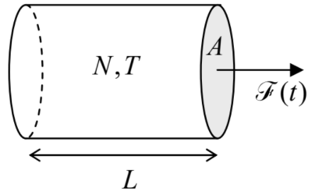
Starting from the Maxwell distribution of velocities, calculate the low-frequency spectral density of fluctuations of the pressure \(P(t)\) of an ideal gas of \(N\) classical particles, in thermal equilibrium at temperature \(T\), and estimate their variance. Compare the former result with the solution of Problem 3.2.

Hints: You may consider a cylindrically-shaped container of volume \(V = LA\) (see the figure on the right), calculate fluctuations of the force \(\mathscr{F}(t)\) exerted by the confined particles on its plane lid of area \(A\), approximating it as a delta-correlated process (\(5.4.17\)), and then re-calculate the fluctuations into those of pressure \(P \equiv \mathscr{F} /A\).

Exercise \(\PageIndex{12}\)

Calculate the low-frequency spectral density of fluctuations of the electric current \(I(t)\) due to the random passage of charged particles between two conducting electrodes – see the figure on the right. Assume that the particles are emitted, at random times, by one of the electrodes, and are fully absorbed by the counterpart electrode. Can your result be mapped on some aspect of the electromagnetic blackbody radiation?

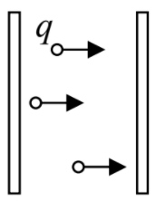
Hint: For the current \(I(t)\), use the same delta-correlated-process approximation as for the force \(\mathscr{F}(t)\) in the previous problem.

Exercise \(\PageIndex{13}\)⁷⁹

A very long, uniform string, of mass \(\mu\) per unit length, is attached to a firm support, and stretched with a constant force (“tension”) \(\mathscr{T}\) – see the figure on the right.

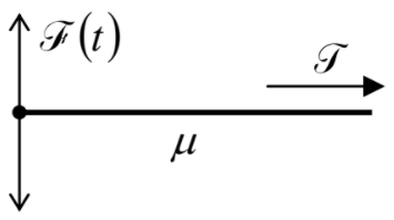
Calculate the spectral density of the random force \(\pmb{\mathscr{F}}(t)\) exerted by the string on the support point, within the plane normal to its length, in thermal equilibrium at temperature \(T\).

Hint: You may assume that the string is so long that a transverse wave, propagating along it from the support point, never comes back.

Exercise \(\PageIndex{14}\)⁸⁰

Each of two 3D harmonic oscillators, with mass \(m\), resonance frequency \(\omega_0\), and damping \(\delta > 0\), has electric dipole moment \(\mathbf{d} = q\mathbf{s}\), where \(\mathbf{s}\) is the vector of oscillator's displacement from its equilibrium position. Use the Langevin formalism to calculate the average potential of electrostatic interaction of these two oscillators (a particular case of the so-called London dispersion force), separated by distance \(r >> (T/m)^{1/2} /\omega_0\), in thermal equilibrium at temperature \(T >> \hbar \omega_0\). Also, explain why the approach used to solve a very similar Problem 2.15 is not directly applicable to this case.

Hint: You may like to use the following integral: \(\int^{\infty}_0 \frac{1-\xi^2}{\left[(1-\xi^2)^2 + (a\xi )^2 \right]^2} d\xi = \frac{\pi}{4a}\).

Exercise \(\PageIndex{15}^*\)

Within the van der Pol approximation,⁸¹ calculate major statistical properties of fluctuations of classical self-oscillations, at:

1. the free (“autonomous”) run of the oscillator, and
2. their phase been locked by an external sinusoidal force,

assuming that the fluctuations are caused by a weak external noise with a smooth spectral density \(S_f(\omega )\). In particular, calculate the self-oscillation linewidth.

Exercise \(\PageIndex{16}\)

Calculate the correlation function of the coordinate of a 1D harmonic oscillator with small Ohmic damping at thermal equilibrium. Compare the result with that for the autonomous self-oscillator (the subject of the previous problem).

Exercise \(\PageIndex{17}\)

Consider a very long, uniform, two-wire transmission line (see the figure on the right) with wave impedance \(\mathscr{Z}\), which allows propagation of TEM electromagnetic waves with negligible attenuation, in thermal equilibrium at temperature \(T\). Calculate the variance \(\langle \mathscr{V}^2\rangle_{\Delta \nu}\) of the voltage \(\mathscr{V}\) between the wires within a small interval \(\Delta \nu\) of cyclic frequencies.

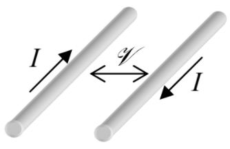
Hint: As an E&M reminder,⁸² in the absence of dispersive materials, TEM waves propagate with a frequency-independent velocity (equal to the speed \(c\) of light, if the wires are in free space), with the voltage \(\mathscr{V}\) and the current \(I\) (see Figure above) related as \(\mathscr{V} (x,t)/I(x,t) = \pm \mathscr{Z}\), where \(\mathscr{Z}\) is line's wave impedance.

Exercise \(\PageIndex{18}\)

Now consider a similar long transmission line but terminated, at one end, with an impedance-matching Ohmic resistor \(R = \mathscr{Z}\). Calculate the variance \(\langle \mathscr{V}^2\rangle_{\Delta \nu}\) of the voltage across the resistor, and discuss the relation between the result and the Nyquist formula (\(5.5.21\)), including numerical factors.

Hint: A termination with resistance \(R = \mathscr{Z}\) absorbs incident TEM waves without reflection.

Exercise \(\PageIndex{19}\)

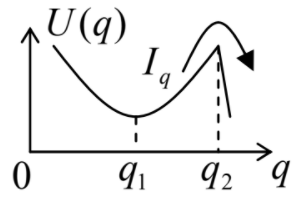
An overdamped classical 1D particle escapes from a potential well with a smooth bottom, but a sharp top of the barrier – see the figure on the right. Perform the necessary modification of the Kramers formula (\(5.6.36\)).

Exercise \(\PageIndex{20}\)

Perhaps the simplest model of the diffusion is the 1D discrete random walk: each time interval \(\tau \), a particle leaps, with equal probability, to any of two adjacent sites of a 1D lattice with spatial period \(a\). Prove that the particle's displacement during a time interval \(t >> \tau\) obeys Equation (\(5.5.16\)), and calculate the corresponding diffusion coefficient \(D\).

Exercise \(\PageIndex{21}\)

A classical particle may occupy any of \(N\) similar sites. Its weak interaction with the environment induces random, incoherent jumps from the occupied site to any other site, with the same time-independent rate \(\Gamma \). Calculate the correlation function and the spectral density of fluctuations of the instant occupancy \(n(t)\) (equal to either 1 or 0) of a site.

---

1. Let me remind the reader that up to this point, the averaging signs \(\langle ...\rangle\) were dropped in most formulas, for the sake of notation simplicity. In this chapter, I have to restore these signs to avoid confusion. The only exception will be temperature – whose average, following (probably, bad :-) tradition, will be still called just \(T\) everywhere, besides the last part of Sec. 3, where temperature fluctuations are discussed explicitly.
2. Unfortunately, even in some popular textbooks, certain formulas pertaining to fluctuations are either incorrect or given without specifying the conditions of their applicability, so that the reader's caution is advised.
3. See, e.g., MA Equation (2.2).
4. It was derived by Jacob Bernoulli (1655-1705).
5. Indeed, this is just the most popular definition of that major mathematical constant – see, e.g., MA Equation (1.2a) with \(n = –1/W\).
6. Named after the same Siméon Denis Poisson (1781-1840) who is also responsible for other mathematical tools and results used in this series, including the Poisson equation – see Sec. 6.4 below.
7. Named after Carl Friedrich Gauss (1777-1855), though Pierre-Simone Laplace (1749-1827) is credited for substantial contributions to its development.
8. As a math reminder, the term “cylinder” does not necessarily mean the “circular cylinder”; the shape of its base may be arbitrary; it just should not change with height.
9. As already was discussed in Sec. 4.1 in the context of the van der Waals equation, for the mechanical stability of a gas (or liquid), the derivative \(\partial P/\partial V\) has to be negative, so that \(\kappa\) is positive.
10. One may meet statements that a similar formula, \[\langle \tilde{P}^2 \rangle_X = T\left(-\frac{\partial \langle P \rangle}{\partial \langle V \rangle}\right)_X, \tag{WRONG!}\] is valid for pressure fluctuations. However, a such statement does not take into account a different physical nature of pressure (Figure \(5.3.1\)), with its very broad frequency spectrum. This issue will be discussed later in this chapter.
11. In this case, we may also use the second of Eqs. (\(1.4.16\)) to rewrite Equation (\(5.3.4-5.3.5\)) via the second derivative \((\partial^2G/\partial P^2)_T\).
12. Besides low internal electric noise, a good sensor should have a sufficiently large temperature responsivity \(dR/dT\), making the noise contribution by the readout electronics insignificant – see below.
13. An important modern trend in this progress [see, e.g., P. Day et al., Nature 425, 817 (2003)] is the replacement of the resistive temperature sensors \(R(T)\) with thin and narrow superconducting strips with temperature-sensitive kinetic inductance \(L_k(T)\) – see the model solution of EM Problem 6.19. Such inductive sensors have zero dc resistance, and hence vanishing Johnson-Nyquist noise at typical signal pickup frequencies of a few kHz – see Equation (\(5.5.20-5.5.22\)) and its discussion below.
14. It was pioneered in the 1950s by Robert Henry Dicke, so that the device is frequently called the Dicke radiometer. Note that the optimal strategy of using similar devices for time- and energy-resolved detection of single high-energy photons is different – though even it is essentially based on Equation (\(5.3.9\)). For a recent brief review of such detectors see, e.g., K. Morgan, Phys. Today 71, 29 (Aug. 2018), and references therein.
15. Another term, the autocorrelation function, is sometimes used for the average (\(5.4.3\)) to distinguish it from the mutual correlation function, \(\langle f_1(t)f_2(t + \tau )\rangle \), of two different stationary processes.
16. Please notice that this correlation function is the direct temporal analog of the spatial correlation function briefly discussed in Sec. 4.2 – see Equation (\(4.2.10\)).
17. Note that the correlation time \(\tau_c\) is the direct temporal analog of the correlation radius \(r_c\) that was discussed in Sec. 4.2 – see the same Equation (\(4.2.10\)).
18. The argument of the function \(f\omega\) is represented as its index with a purpose to emphasize that this function is different from \(\tilde{f}(t)\), while (very conveniently) still using the same letter for the same variable.
19. See, e.g., MA Equation (14.4).
20. The second form of Equation (\(5.4.14\)) uses the fact that, according to Equation (\(5.4.13\)), \(S_f(\omega )\) is an even function of frequency – just as \(K_f(\tau )\) is an even function of time.
21. Although Eqs. (\(5.4.13\)) and (\(5.4.14\)) look not much more than straightforward corollaries of the Fourier transform, they bear a special name of the Wiener-Khinchin theorem – after the mathematicians N. Wiener and A. Khinchin who have proved that these relations are valid even for the functions \(f(t)\) that are not square-integrable, so that from the point of view of standard mathematics, their Fourier transforms are not well defined.
22. Such process is frequently called the white noise, because it consists of all frequency components with equal amplitudes, reminding the white light, which consists of many monochromatic components with close amplitudes.
23. To emphasize this generality, in the forthcoming discussion of the 1D case, I will use the letter \(q\) rather than \(x\) for the system's displacement.
24. For a usual (ergodic) environment, the primary averaging may be interpreted as that over relatively short time intervals, \(\tau_c << \Delta t << \tau \), where \(\tau_c\) is the correlation time of the environment, while \(\tau\) is the characteristic time scale of motion of our “heavy” system of interest.
25. Named after Paul Langevin, whose 1908 work was the first systematic development of A. Einstein's ideas on Brownian motion (see below) using this formalism. A detailed discussion of this approach, with numerical examples of its application, may be found, e.g., in the monograph by W. Coffey, Yu. Kalmykov, and J. Waldron, The Langevin Equation, World Scientific, 1996.
26. See, e.g., CM Sec. 5.1. Here I assume that the variable \(f(t)\) is classical, with the discussion of the quantum case postponed until the end of the section.
27. Note that the direct secondary statistical averaging of Equation (\(5.5.3\)) with \(\mathscr{F}_{det} = 0\) yields \(\langle \langle q\rangle \rangle = 0!\) This, perhaps a bit counter-intuitive result becomes less puzzling if we recognize that this is the averaging over a large statistical ensemble of random sinusoidal oscillations with all values of their phase, and that the (equally probable) oscillations with opposite phases give mutually canceling contributions to the sum in Equation (\(2.1.6\)).
28. At this stage, we restrict our analysis to random, stationary processes \(q(t)\), so that Equation (\(5.4.12\)) is valid for this variable as well, if the averaging in it is understood in the \(\langle \langle ...\rangle \rangle\) sense.
29. Regardless of the physical sense of such a function of \(\omega \), and of whether its maximum is situated at a finite frequency \(\omega_0\) as in Equation (\(5.5.6\)) or at \(\omega = 0\), it is often referred to as the Lorentzian (or “Breit-Wigner”) line.
30. Since in this case the process in the oscillator is entirely due to its environment, its variance should be obtained by statistical averaging over an ensemble of many similar (oscillator + environment) systems, and hence, following our convention, it is denoted by double angular brackets.
31. See, e.g. MA Equation (6.5a).
32. See, e.g., CM Sec. 5.1.
33. It was published in one of the three papers of Einstein's celebrated 1905 “triad”. As a reminder, another paper started the (special) relativity theory, and one more was the quantum description of the photoelectric effect, essentially starting the quantum mechanics. Not too bad for one year, one young scientist!
34. In particular, in 1908, i.e. very soon after Einstein's publication, it was used by J. Perrin for an accurate determination of the Avogadro number \(N_A\). (It was Perrin who graciously suggested naming this constant after A. Avogadro, honoring his pioneering studies of gases in the 1810s.)
35. Note that in solid-state physics and electronics, the charge carrier mobility is usually defined as \(| \mathbf{v}_{drift}/\pmb{\mathscr{E}} | = e\mathbf{v}_{drift}/|\pmb{\mathscr{F}}_{det}| \equiv e| \mu |\) (where \(\pmb{\mathscr{E}}\) is the applied electric field), and is traditionally measured in cm\(^2\)/V\(\cdot\)s.
36. The minus sign is due to the fact that in our notation, the current flowing in the resistor, from the positive terminal to the negative one, is (\(-I\)) – see Figure \(5.5.1\).
37. Due to this fact, Equation (\(5.5.2\)) is often called the Ohmic model of the environment's response, even if the physical nature of the variables \(q\) and \(\mathscr{F}\) is completely different from the electric charge and voltage.
38. It is named after Harry Nyquist who derived this formula in 1928 (independently of the prior work by A. Einstein, M. Smoluchowski, and P. Langevin) to describe the noise that had been just discovered experimentally by his Bell Labs' colleague John Bertrand Johnson. The derivation of Equation (\(5.5.11-5.5.12\)) and hence Equation (\(5.5.20-5.5.22\)) in these notes is essentially a twist of the derivation used by H. Nyquist.
39. See, e.g., J. Crossno et al., Appl. Phys. Lett. 106, 023121 (2015), and references therein.
40. Another practically important type of fluctuations in electronic devices is the low-frequency \(1/f\) noise that was already mentioned in Sec. 3 above. I will briefly discuss it in Sec. 8.
41. It was derived by Walter Hans Schottky as early as 1918, i.e. even before Nyquist's work.
42. See, e.g., Y. Naveh et al., Phys. Rev. B 58, 15371 (1998). In practically used metals, \(l_e\) is of the order of 30 nm even at liquid-helium temperatures (and much shorter at room temperatures), so that the usual “macroscopic” resistors do not exhibit the shot noise.
43. For a review of this effect see, e.g., Ya. Blanter and M. Büttiker, Phys. Repts. 336, 1 (2000).
44. See, e.g., a concise book by A. Balbi, The Music of the Big Bang, Springer, 2008.
45. Reviewing the calculations leading to Equation (\(5.5.11-5.5.12\)), we may see that the possible real part \(\chi '(\omega )\) of the susceptibility just adds up to \((k – m\omega^2)\) in the denominator of Equation (\(5.5.5\)), resulting in a change of the oscillator's frequency \(\omega_0\). This renormalization is insignificant if the oscillator-to-environment coupling is weak, i.e. if the susceptibility \(\chi (\omega )\) is small – as had been assumed at the derivation of Equation (\(5.5.7\)) and hence Equation (\(5.5.11-5.5.12\)).
46. It is sometimes called the Green-Kubo (or just the Kubo) formula. This is hardly fair, because, as the reader could see, Equation (\(5.5.33\)) is just an elementary generalization of the Nyquist formula (\(5.5.20-5.5.22\)). Moreover, the corresponding works of M. Green and R. Kubo were published, respectively, in 1954 and 1957, i.e. after the 1951 paper by H. Callen and T. Welton, where a more general result (\(5.5.39\)) had been derived. Much more adequately, the Green/Kubo names are associated with Equation (\(5.5.43\)) below.
47. See, e.g., QM Sec. 4.6.
48. Here (and to the end of this section) the averaging \(\langle ...\rangle\) should be understood in the general quantum-statistical sense – see Equation (\(2.1.12\)). As was discussed in Sec. 2.1, for the classical-mixture state of the system, this does not create any difference in either the mathematical treatment of the averages or their physical interpretation.
49. R. Koch et al., Phys. Rev. B 26, 74 (1982), and references therein.
50. See, e.g., QM Sec. 7.4.
51. See, e.g., CM Sec. 5.1.
52. See, e.g., CM Secs. 3.4-3.6.
53. The generalization of Equation (\(5.6.1\)) to higher spatial dimensionality is also straightforward, with the scalar variable \(q\) replaced with a multi-dimensional vector \(\mathbf{q}\), and the scalar derivative \(dU/dq\) replaced with the vector \(\nabla U\), where \(\nabla\) is the del vector-operator in the \(\mathbf{q}\)-space.
54. See, e.g., CM Secs. 3.2, 5.2, and beyond.
55. See, e.g., QM Problem 7.8, and also Chapters 5 and 6 in the monograph by W. Coffey et al., cited above.
56. It was named after Hendrik Anthony (“Hans”) Kramers who, besides solving this conceptually important problem in 1940, has made several other seminal contributions to physics, including the famous Kramers-Kronig dispersion relations (see, e.g., EM Sec. 7.4) and the WKB (Wentzel-Kramers-Brillouin) approximation in quantum mechanics – see, e.g., QM Sec. 2.4.
57. If \(U_0\) is comparable with \(T\), the system's behavior also depends substantially on the initial probability distribution, i.e., does not follow the simple law (\(5.6.5-5.6.6\)).
58. See, e.g., either R. Stratonovich, Topics in the Theory of Random Noise, vol. 1., Gordon and Breach, 1963, or Chapter 1 in the monograph by W. Coffey et al., cited above.
59. By the way, the goal of the traditional definition (\(5.5.17\)) of the diffusion coefficient, leading to the front coefficient 2 in Equation (\(5.5.16\)), is exactly to have the fundamental equations (\(5.6.9\)) and (\(5.6.11\)) free of numerical coefficients.
60. As will be discussed in Chapter 6, the equation of diffusion also describes several other physical phenomena – in particular, the heat propagation in a uniform, isotropic solid, and in this context is called the heat conduction equation or (rather inappropriately) just the “heat equation”.
61. Both forms of Equation (\(5.6.12-5.6.13\)) are similar to the mass conservation law in classical dynamics (see, e.g., CM Sec. 8.2), the electric charge conservation law in electrodynamics (see, e.g., EM Sec. 4.1), and the probability conservation law in quantum mechanics (see, e.g., QM Sec. 1.4).
62. See, e.g., MA Equation (12.2),
63. It is named after Marian Smoluchowski, who developed this formalism in 1906, apparently independently from the slightly earlier Einstein's work, but in much more detail. This equation has important applications in many fields of science – including such surprising topics as statistics of spikes in neural networks. (Note, however, that in some non-physical fields, Equation (\(5.6.18\)) is referred to as the Fokker-Planck equation, while actually, the latter equation is much more general – see the next section.)
64. If necessary, see MA Equation (6.9b) again.
65. Actually, \(\tau_2\) describes the characteristic time of the exponential growth of small deviations from the unstable fixed point \(q_2\) at the barrier top, rather than their decay, as near the stable point \(q_1\).
66. It was first derived by Adriaan Fokker in 1913 in his PhD thesis, and further elaborated by Max Planck in 1917. (Curiously, A. Fokker is more famous for his work on music theory, and the invention and construction of several new keyboard instruments, than for this and several other important contributions to theoretical physics.)
67. An example of such an equation, for the particular case of a harmonic oscillator, is given by QM Equation (7.214). The Fokker-Planck equation, of course, can give only its classical limit, with \(n, n_e >> 1\).
68. A detailed description of this calculation (first performed by H. Kramers in 1940) may be found, for example, in Sec. III.7 of the review paper by S. Chandrasekhar, Rev. Mod. Phys. 15, 1 (1943).
69. See, e.g., QM Secs. 2.4-2.6.
70. As a reminder, a similar approximation arises for the \(P(V)\) function, at the analysis of the van der Waals model near the critical temperature – see Problem 4.6.
71. The main, exponential factor in this result may be obtained simply by ignoring the difference between \(E\) and \(U(q_1)\), but the correct calculation of the pre-exponential factor requires taking this difference, \(\hbar \omega_0/2\), into account – see, e.g., the model solution of QM Problem 2.43.
72. See, e.g., QM Sec. 2.4.
73. The step from the first line of Equation (\(5.8.10\)) to its second line utilizes the fact that our system is stationary, so that \(\langle E(t + \tau )\rangle = \langle E(t)\rangle = \langle E(\infty )\rangle =\) const.
74. See, e.g., MA Equation (6.9c).
75. The involved table integral may be found, e.g., in MA Equation (6.11).
76. See, e.g., QM Sec. 7.6.
77. See, e.g., the solutions of the 1D Kramers problem for quantum systems with low damping by A. Caldeira and A. Leggett, Phys. Rev. Lett. 46, 211 (1981), and with high damping by A. Larkin and Yu. Ovchinnikov, JETP Lett. 37, 382 (1983).
78. Note that these two cases may be considered as the non-interacting limits of, respectively, the Ising model (\(4.2.3\)) and the classical limit of the Heisenberg model (\(4.2.1\)), whose analysis within the Weiss approximation was the subject of Problem 4.18.
79. This problem, conceptually important for the quantum mechanics of open systems, was given in Chapter 7 of the QM part of this series, and is repeated here for the benefit of the readers who, by any reason, skipped that course.
80. This problem, for the case of arbitrary temperature, was the subject of QM Problem 7.6, with Problem 5.15 of that course serving as the background. However, the method used in the model solutions of those problems requires one to prescribe, to the oscillators, different frequencies \(\omega_1\) and \(\omega_2\) at first, and only after this more general problem has been solved, pursue the limit \(\omega_1 \rightarrow \omega_2\), while neglecting dissipation altogether. The goal of this problem is to show that the result of that solution is valid even at non-zero damping.
81. See, e.g., CM Secs. 5.2-5.5. Note that in quantum mechanics, a similar approach is called the rotating-wave approximation (RWA) – see, e.g., QM Secs. 6.5, 7.6, 9.2, and 9.4.
82. See, e.g., EM Sec. 7.6.