
14.3: Waves on a Rope


- Last updated
- Jul 6, 2024
- Save as PDF
( \newcommand{\kernel}{\mathrm{null}\,}\)
In this section, we model the motion of transverse waves on a rope, as this provides insight into many properties of waves that extend to waves propagating in other media.
A pulse on a rope
We start by modeling how a single pulse propagates down a horizontal rope that is under a tension, FT1. A wave is generally considered to be a regular series of alternating upwards and downwards pulses propagating down the rope. Modeling the propagation of a pulse is thus equivalent to modeling the propagation of a wave. Figure 14.3.1 shows how one can generate a pulse in a taught horizontal rope by raising (and then lowering) one end of the rope.
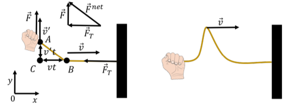
We can model the propagation speed of the pulse by considering the speed, v, of point B that is shown in the left panel of Figure 14.3.1. Note that point B is not a particle of the rope, and is, instead, the location of the “front” of the disturbance that the pulse causes on the rope. We model the rope as being under a horizontal force of tension, →FT, and the pulse is started by exerting a vertical force, →F, to move the end (point A) of the rope upwards with a speed, v′. Thus, by pulling upwards on the rope with a force, →F, at a speed v′, we can start a disturbance in the rope that will propagate with speed v.
In a short amount of time, t, the point A on the rope will have moved up by a distance v′t, whereas point B will have moved to the right by a distance vt. If t is small enough, we can consider the points A, B, and C to form the corners of a triangle. That triangle is similar to the triangle that is made by vectorially summing the applied force →F and the tension →FT, as shown in the top left of Figure 14.3.1. In this case, we mean the geometry term “similar”, which describes two triangles which have the same angles. We can thus write:
\[\begin{aligned} \frac{F}{F_T}&=\frac{v't}{vt}=\frac{v'}{v}\
\boldsymbol{4pt] \therefore F&= F_T \frac{v'}{v}\end{aligned}}
Consider the section of rope with length vt that we have raised by applying that force (we assume that the distance AB is approximately equal to the distance BC). If the rope has a mass per unit length μ, then the mass of the rope element that was raised (between points A and B) has a mass, m, given by:
m=μvt
The vertical component of the momentum of that section of rope, with vertical speed given by v′, is thus:
p=mv′=μvtv′
If the vertical force, →F, was exerted for a length of time, t, on the mass element, it will give it a vertical impulse, Ft, equal to the change in the vertical momentum of the mass element:
\[\begin{aligned} Ft &= \Delta p \
\[4pt] Ft &= \mu vt v'\
\boldsymbol{4pt] \therefore F &= \mu v v'\end{aligned}}
We can equate this expression for F with that obtained from the similar triangles to obtain an expression for the speed, v, of the pulse:
\[\begin{aligned} \mu v v' &= F_T \frac{v'}{v}\
\boldsymbol{4pt] \therefore v&= \sqrt{\frac{F_T}{\mu}}\end{aligned}}
The speed of a pulse (and wave) propagating through a rope with linear mass density, μ, under a tension, FT, is given by:
v=√FTμ
If the tension in the rope is higher, the pulse will propagate faster. If the linear mass density of the rope is higher, then the pulse will propagate slower.
Reflection and transmission
In this section, we examine what happens when a pulse traveling down a rope arrives at the end of the rope. First, consider the case illustrated in Figure 14.3.2 where the end of the rope is fixed to a wall.
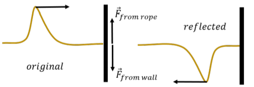
When the pulse arrives at the wall, the rope will exert an upwards force on the wall, →Ffromrope. By Newton’s Third Law, the wall will then exert a downwards force on the rope, →Ffromwall. The downwards force exerted on the rope will cause a downwards pulse to form, and the reflected pulse will be inverted compared to the initial pulse that arrived at the wall.
Now, consider the case when the end of the rope has a ring attached to it, so that it can slide freely up and down a post, as illustrated in Figure 14.3.3.
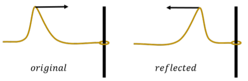
In this case, the end of the rope will move up as the pulse arrives, which will then create a reflected pulse that is in the same orientation as the incoming pulse.
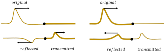
Finally, consider a pulse that propagates down a rope of mass per unit length μ1 that is tied to a second rope with mass per unit length μ2, which have the same tension. When the pulse arrives at the interface between the two media (the two ropes), part of the pulse will be reflected back, and part will be transmitted into the second medium (Figure 14.3.4).
By considering the boundary conditions, one can derive the coefficient of reflection, R (see Exercise 14.10.2 for the derivation). This coefficient is the ratio of the amplitude of the reflected pulse to the amplitude of initial pulse. The ratio is found to be:
R=√μ1−√μ2√μ1+√μ2
When the pulse moves from a lighter rope to a heavier rope (μ1<μ2), the reflected pulse will be inverted (R<0). When the pulse moves from a heavier rope to a lighter rope (μ1>μ2), the reflected pulse will stay upright (R>0).
When the end of the rope is fixed to a wall (as in Figure 14.3.2), this represents a limiting case in which the linear mass density of the second material approaches infinity (μ2→∞):
R=limμ2→∞√μ1−√μ2√μ1+√μ2=−√μ2√μ2=−1
which means that the amplitude of the reflected pulse will have the same magnitude as the initial pulse but will be in the opposite direction. When the end of the rope is free (Figure 14.3.3), this represents another limiting case, where μ2→0:
R=limμ2→0√μ1−√μ2√μ1+√μ2=√μ1√μ1=1
which means that the amplitude of the reflected pulse will be in the same direction and have the same amplitude as the initial pulse.
A wave propagates from a light rope to a heavier rope that is attached to the light rope (as the pulse illustrated in Figure 14.3.4). What can you say about the wavelength of the wave on either side of the interface?
- It is the same in both sections of rope.
- The wavelength in the heavy section of rope is longer.
- The wavelength in the light section of rope is longer.
- Answer
- C.
The wave equation for a rope
In this section, we show how to use Newton’s Second Law to derive the wave equation for transverse waves traveling down a rope with linear mass density, μ, under a tension, FT. Consider a small section of the rope, with mass dm, and length dx, as a wave passes through that section of the rope, as illustrated in Figure 14.3.5.
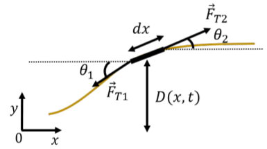
We assume that the weight of the mass element is negligible compared to the force of tension that is in the rope. Thus, the only forces exerted on the mass element are those from the tension in the rope, pulling on the mass element from each side, with forces, →FT1 and →FT2. In general, the forces from tension on either side of the mass element will have different directions and make different angles, θ, with the horizontal, although their magnitude is the same. Let D(x,t) be the vertical displacement of the mass element located at position x. We can write the y (vertical) component of Newton’s Second Law for the mass element, dm, as:
\[\begin{aligned} \sum F_y = F_{T2y} - F_{T1y} &= (dm)a_y\
\[4pt] F_T\sin\theta_2 - F_T\sin\theta_1 &= dm \frac{\partial ^{2}D}{\partial t^{2}}\
\boldsymbol{4pt] F_T(\sin\theta_2 - \sin\theta_1) &= dm \frac{\partial ^{2}D}{\partial t^{2}}\end{aligned}}
where we used the fact that the force of tension has a magnitude, FT, on either side of the mass element, and that the acceleration of the mass in the vertical direction is the second time-derivative of D(x,t), since for a transverse wave, this corresponds to the y position of a particle. We now make the small angle approximation:
sinθ≈tanθ=∂D∂x
in which the sine of the angle is approximately equal to the tangent of the angle, which is equal to the slope of the rope. Applying this approximation to Newton’s Second Law:
FT(∂D∂x|right−∂D∂x|left)=dm∂2D∂t2
where we indicated that the term in parentheses is the difference in the slope of the rope between the right side and the left side of the mass element. If the rope has linear mass density, μ, then the mass of the rope element can be expressed in terms of its length, dx:
dm=μdx
Replacing dm in the equation gives:
\[\begin{aligned} F_T\left(\frac{\partial D}{\partial x}\Bigr|_{right} - \frac{\partial D}{\partial x}\Bigr|_{left}\right) &= \mu dx \frac{\partial ^{2}D}{\partial t^{2}}\
\boldsymbol{4pt] F_T\left(\frac{\frac{\partial D}{\partial x}\Bigr|_{right} - \frac{\partial D}{\partial x}\Bigr|_{left}}{dx}\right) &= \mu \frac{\partial ^{2}D}{\partial t^{2}}\end{aligned}}
The term in parentheses is the difference in the first derivatives of D(x,t) with respect to x, divided by the distance, dx, between which those derivatives are evaluated. This is precisely the definition of the second derivative with respect to x, so we can write:
\[\begin{aligned} F_T \frac{\partial ^{2}D}{\partial x^{2}} &= \mu \frac{\partial ^{2}D}{\partial t^{2}}\
\[4pt] \therefore \frac{\partial ^{2}D}{\partial x^{2}} &= \frac{\mu}{F_T} \frac{\partial ^{2}D}{\partial t^{2}}\
\boldsymbol{4pt]\end{aligned}}
which is precisely the wave equation:
\[\begin{aligned} \frac{\partial ^{2}D}{\partial x^{2}} &= \frac{1}{v^2} \frac{\partial ^{2}D}{\partial t^{2}}\
\boldsymbol{4pt]\end{aligned}}
with speed:
v=√FTμ
as we found earlier. Thus, we find that the speed of the propagation of the wave is related to the dynamics of modeling the system, and is not related to the wave itself.
Footnotes
1. We do not use T for tension, so as to not confuse with the period of a wave.