20.2: Kirchhoff’s rules
- Page ID
- 19515
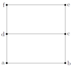
Kirchhoff’s rules correspond to concepts that we have already covered, but allow us to easily model more complex circuits, for instance, those where there is more than one path for the current to take. Kirchhoff’s rules refer to “junctions” and “loops”. Junctions and loops depend only on the shape of the circuit, and not on the components in the circuit. Figure \(\PageIndex{1}\) shows a circuit with no components in order to illustrate what is meant by a junction and a loop.

The locations at points \(d\) and \(c\) are considered “junctions”, because there are more than \(2\) segments of wire connected to that point. The points at locations \(a\), \(b\), \(e\) and \(f\) only have two segments of wire connected to them. The circuit in Figure \(\PageIndex{1}\) thus has \(2\) junctions.
A loop is a closed path that one can trace around the circuit without passing over the same segment of wire twice. The circuit in Figure \(\PageIndex{1}\) has \(3\) such loops, which we can identify using the letters at the various nodes of the circuit:
- \(abcda\)
- \(abcefda\)
- \(dcefd\)
Note that it does not matter where one starts on the loop, only that one can identify how many different loops are present in the circuit.

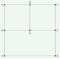
How many loops and junctions does the circuit in Figure \(\PageIndex{2}\) have?
- The circuit has five loops and four junctions
- The circuit has three loops and eight junctions
- The circuit has seven loops and four junctions.
- The circuit has four loops and four junctions.
- Answer
Junction Rule
The junction rule states that: The current entering a junction must be equal to the current exiting a junction.
This is in fact a simple statement about conservation of charge. If charges are flowing into a junction (from one or more segments of wire in that junction), then the same amount of charges must flow back out of the junction (through one or more different segments of wire).
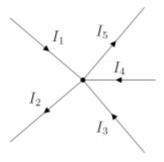
Consider the junction illustrated in Figure \(\PageIndex{3}\), comprised of \(5\) segments of wire, each carrying a different current. As shown, currents \(I_1\) and \(I_4\) flow into the junction, whereas currents \(I_2\), \(I_3\) and \(I_5\) all flow out of the junction.

The junction rule states that the current entering the junction must equal the current coming out of the junction. This allows us to relate the currents to each other in an equation:
\[\begin{aligned} \text{incoming currents}&=\text{outgoing currents}\\[4pt] I_1+I_4 &=I_2+I_3+I_4\end{aligned}\]
Loop Rule
The loop rule states that: The net voltage drop across a loop must be zero.
This is a statement about conservation of energy, that we already noted in Example 20.1.1. Once you have identified a specific loop, if you trace a closed path around the loop, the electric potential must be the same at the end of the path as at the beginning of the path (since it is literally the same point in space). This means that if there is a voltage drop along the path (e.g. due to one or more resistors), then there must be equivalent voltage increases somewhere else on the path (e.g. due to one or more batteries). If this were not the case, it would be possible to have a path where charges could gain a net amount of energy by going around that path, which they could keep doing indefinitely and create an infinite amount of energy; instead, if charges gain potential energy in a battery, they must then loose exactly the same amount of energy inside one or more resistors along the path.
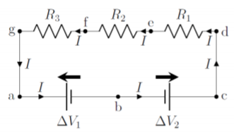
Figure \(\PageIndex{4}\) shows a loop (which could be part of a larger circuit) to which we can apply the loop rule. The loop contains two batteries, facing in opposite directions (which would not normally be a good use of batteries), as illustrated by the battery arrows.

The procedure for applying the loop rule is as follows:
- Identify the loop, including starting position and direction.
- Start at the beginning of the loop, and trace around the loop.
- Each time a battery is encountered, add the battery voltage if you are tracing the loop in the same direction as the corresponding battery arrow, subtract the voltage otherwise.
- Each time a resistor is encountered, subtract the voltage across that resistor (\(RI\), from Ohm’s Law) if tracing the loop in the same direction as the current, add the the voltage otherwise.
- Once you have traced back to the starting point, the resulting sum must be zero.
To illustrate the procedure, we trace out the loop \(abcedfga\) in Figure \(\PageIndex{4}\). We thus start at point \(a\) and trace the loop in the counter-clockwise direction.
- Between points \(a\) and \(b\) we encounter a battery, and we are tracing in the opposite direction of that battery’s arrow, so we subtract the voltage from that battery: \(-\Delta V_1\).
- Between points \(b\) and \(c\), we encounter a battery, and we are tracing in the same direction as that battery’s arrow, so we add the voltage from that battery: \(+\Delta V_2\).
- Nothing happens to the potential along the wire from \(c\) to \(d\).
- Between points \(d\) and \(e\), we encounter a resistor, and we are tracing in the same direction as the current through that resistor, so subtract the voltage across that resistor: \(-R_1I\)).
- Similarly, we subtract the voltages across resistors \(R_2\) and \(R_3\), as we are tracing in the same direction as the current through those resistors: \(-IR_2-IR_3\).
- We are back at the beginning of the loop, so the terms must sum to zero.
We can now use the loop rule, which states that the sum of the above voltages must be zero:
\[\begin{aligned} -\Delta V_1 + \Delta V_2 - R_1I - R_2I - R_3I = 0\quad \text{(loop abcdefga)}\end{aligned}\]
This equation then gives us a relation between the various quantities (current, resistors, battery voltages) in the circuit which can be used to model the circuit.
Suppose that the equation describing loop \(abcdefga\) (Figure \(\PageIndex{4}\)) was obtained from a different starting position and the loop was traced in the opposite direction. Would this produce a different equation?
- Yes, the equation would be incorrect if the loop is traced in the direction opposite to the flow of current.
- Yes, the equation must start from the point \(a\) because the creator of the circuit assumes the person calculating current and voltage will begin at point \(a\).
- Yes, there is no incorrect starting point, but choosing to trace the circuit in the direction opposite to the flow of current would produce an incorrect equation.
- No, there is no incorrect direction or starting point.
- Answer

