25.2: Vectors
( \newcommand{\kernel}{\mathrm{null}\,}\)
So far, we have seen how to use a coordinate system to describe the position of a single point in space relative to an origin. In this section, we introduce the notion of a “vector”, which allows us to describe quantities that have a magnitude and a direction. For example, you can use a vector to describe the fact that you walked 5 km in the North direction. A vector can be visualized by an arrow. The length of the arrow is the magnitude that we wish to describe, and the direction of the arrow corresponds to the direction that we would like to describe.
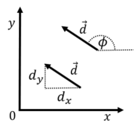
Unlike a point in space, vectors have no location. That is, vectors are simply an arrow, and you can choose to draw that arrow anywhere you like. In two dimensional space, one requires two numbers to completely define a vector. In three dimensional space, one requires three numbers to completely define a vector. Figure A1.2.1 shows a two dimensional vector, →d, twice. Because both arrows in the figure have the same magnitude and direction, they represent the same vector. When we refer to quantities that are vectors, we usually draw an arrow on top of the quantity (→d) to indicate that they are vectors. We use the word “scalar” to refer to numbers that are not vectors (a regular number is thus also called a scalar to distinguish it from a quantity that is a vector).

In analogy with coordinate systems, we have multiple ways to choose the numbers that we use to describe the vector. The most convenient choice is usually to use the “Cartesian components” of the vector which correspond to the length of the vector when projected onto a Cartesian coordinate system. For example, in Figure A1.2.1, the Cartesian components of the vector \vec d are labeled as (d_x, d_y) indicating that the vector has a length of d_x in the x direction and d_y in the y direction. Furthermore, the number d_x is negative, since the vector points in the negative x direction. Another common choice is to use the length of the vector, which we label d (the name of the vector without the arrow on top), and the angle, \phi that the vector makes with the x-axis, as illustrated in Figure A1.2.1. In terms of the two dimensional Cartesian components, the magnitude of the vector is given by:
\begin{aligned} d&= ||\vec d||= \sqrt{d_x^2+d_y^2}\end{aligned}
where we also introduced the notation that placing two vertical bars around a vector (||\vec d||) is used to indicated its magnitude. Note that in three dimensions, it is usually not convenient to specify the direction unless the vector lies in one of the planes defined by the coordinate system (e.g the xy plane). In three dimensions, it is usually most convenient to specify the three Cartesian components.
Unit vectors
A special category of vectors is “unit vectors”, which are simply vectors that have a length (magnitude) of 1 (in whichever units the coordinate system is defined). Unit vectors are particularly useful for indicating direction. For example, in Figure A1.2.1, we may be interested in indicating the direction of the vector \vec d. Unit vectors are denoted by using a “hat” instead of an arrow. Thus, the vector \hat d, is the vector of length 1 that points in the same direction as \vec d. The (Cartesian) components of \hat d are easily found by dividing the corresponding components of \vec d by d (the magnitude):
\begin{aligned} (\hat d)_x &= \frac{d_x}{d}=\frac{d_x}{\sqrt{d_x^2+d_y^2}}\\[4pt] (\hat d)_y &= \frac{d_y}{d}=\frac{d_y}{\sqrt{d_x^2+d_y^2}}\\[4pt] \therefore d &= ||\hat d||=\sqrt{(\hat d)_x^2+(\hat d)_y^2}=\sqrt{\frac{d_x^2}{d_x^2+d_y^2}+\frac{d_y^2}{d_x^2+d_y^2}}=1\end{aligned}
A specific type of unit vector is the units vectors that are parallel to the axes of the coordinate system. Those vectors are denoted \hat x, \hat y, \hat z (and sometimes \hat i, \hat j, \hat k or \hat e_x, \hat e_y, \hat e_z) for the x, y, and z axes, respectively. Thus, the vector d\hat{x}, is the vector of length d that points in the positive x direction.
Notations and representation of vectors
There are multiple notations for describing a vector using its components. The following are all equivalent ways to write down the vector \vec d in terms of its components d_x and d_y:
\begin{aligned} \vec d &= (d_x,d_y)\quad&\text{row vector}\\[4pt] &=\begin{pmatrix} d_x \\[4pt] d_y \\[4pt] \end{pmatrix}\quad&\text{column vector}\\[4pt] &= d_x\hat x +d_y \hat y\quad&\text{using }\hat x,\;\hat y\\[4pt] &=d_x\hat i +d_y \hat j \quad&\text{using }\hat i,\;\hat j\end{aligned}
The vectors \hat x (\hat i) and \hat y (\hat j) are unit vectors in x and y directions respectively. For example, the unit vector \hat y can be written down as (0,1) in two dimensions or (0,1,0) in three dimensions, using the row notation.
What is the magnitude (the length) of the vector 5\hat x-2\hat y?
- 3.0
- 5.4
- 7.0
- 10.0
- Answer
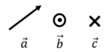
Illustrating a vector graphically in two dimensions is straightforward, but difficult in three dimensions. To help remedy this, a notation is introduced in order to draw vectors that point in or out of the page (perpendicular to the plane of the page). The notation comes from imagining that the vector is an archery arrow. If the vector is coming out of the page (at you!), then you would see the head of the arrow, which we represent as a circle with a dot (the dot is the point of the arrow, the circle is the base of the conically shaped arrowhead). If instead, the vector points into the page, then you would see the back of the arrow, which we represent as a cross (the cross being the feathers in the tail of the arrow). This is illustrated in Figure A1.2.2.


