25.3: Vector algebra

In this section, we describe the various algebraic operations that can be performed using vectors.

Multiplication/division of a vector by a scalar

One can multiply (or divide) a vector by a scalar (a number). Suppose that we are given a vector \(\vec v=(v_x, v_y, v_z)\) and a scalar \(a\). The multiplication \(a\vec v\) is defined to be a new vector, say \(\vec w\), whose components are the components of \(\vec v\) multiplied by \(a\):

\[\begin{aligned} \vec w = a\vec v = (av_x, a v_y, av_z)\end{aligned}\]

Similarly, the division of a vector by a scalar is defined analogously by dividing each Cartesian component by the scalar::

\[\begin{aligned} \vec w = \frac{\vec v}{a} = \left(\frac{v_x}{a}, \frac{v_y}{a}, \frac{v_z}{a}\right)\end{aligned}\]

Exercise \(\PageIndex{1}\)

What happens to the length of a vector if the vector is multiplied by \(2\) (a scalar)?

1. The length doubles
2. The length is halved
3. The length is quadrupled
4. It depends on the direction of the vector

Answer

In particular, this makes it easy to determine the unit vector, \(\hat v\), that points in the same direction as \(\vec v\):

\[\begin{aligned} \hat v = \frac{\vec v}{v}\end{aligned}\]

where \(v\) is the (scalar) magnitude of \(\vec v\).

Addition/subtraction of two vectors

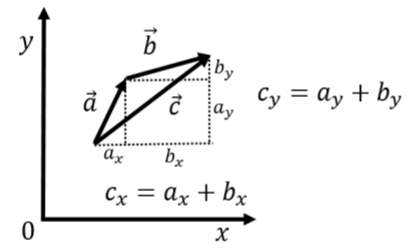
The sum of two vectors, \(\vec a\) and \(\vec b\), is found by adding the components of the two vectors. Similarly, the difference between two vectors is found by subtracting the components. For example, if \(\vec c=\vec a+\vec b\), the components of \(\vec c\) are given by:

\[\begin{aligned} \vec c &= \vec a + \vec b = \begin{pmatrix} a_x \\[4pt] a_y \\[4pt] \end{pmatrix} + \begin{pmatrix} b_x \\[4pt] b_y \\[4pt] \end{pmatrix}\\[4pt] \therefore \begin{pmatrix} c_x \\[4pt] c_y \\[4pt] \end{pmatrix} &=\begin{pmatrix} a_x+b_x \\[4pt] a_y+b_y \\[4pt] \end{pmatrix}\end{aligned}\]

where we chose to use the “column vector” notation. The column vector notation highlights the fact that the algebra (addition, subtraction) is performed independently on the \(x\) and \(y\) components. We can thus use write this sum equivalently as two scalar equations, one for each coordinate:

\[\begin{aligned} c_x &= a_x+b_x\\[4pt] c_y &= a_y+b_y\end{aligned}\]

Vectors can thus be used as a short-hand notation for representing multiple equations (one equation per component). When we use vectors to write an equation such as:

\[\begin{aligned} \vec F = m\vec a\end{aligned}\]

we really mean that there is one scalar equation per component of the vectors:

\[\begin{aligned} F_x &= ma_x\\[4pt] F_y &= ma_y\\[4pt] F_z &= ma_z\end{aligned}\]

Example \(\PageIndex{1}\)

Given two vectors, \(\vec a=2\hat x+3\hat y\), and \(\vec b=5\hat x-2\hat y\), calculate the vector \(\vec c= 2\vec a- 3\vec b\).

Solution

This can easily be solved algebraically by collecting terms for each component, \(\hat x\) and \(\hat y\):

\[\begin{aligned} \vec c &= 2\vec a- 3\vec b\\[4pt] &=2 (2\hat x+3\hat y) - 3 (5\hat x-2\hat y) \\[4pt] &=(4\hat x+6\hat y)-(15\hat x-6\hat y) \\[4pt] &=(4-15)\hat x + (6+6) \hat y\\[4pt] &= -11 \hat x + 12 \hat y\end{aligned}\]

We can think of these operations as being performed independently on the components:

\[\begin{aligned} c_x&=2a_x-3b_x=-11\\[4pt] c_y&=2a_y-3b_y=12\end{aligned}\]

Geometrically, one can easily visualize the addition and subtraction of vectors. This is illustrated in Figure A1.3.1 for the case of adding vectors \(\vec a\) and \(\vec b\) to get the vector \(\vec c\). Geometrically, the sum of the vectors \(\vec a\) and \(\vec b\) (sometimes also called the “resultant”) can be found by:

1. Placing the “tail” of vector \(\vec b\) at the “head” of \(\vec a\) (think of an arrow, the pointy part is the head and the feathery part is the tail)
2. Drawing the vector that goes from the tail of vector \(\vec a\) to the head of vector \(\vec b\).

Figure A1.3.1: Geometric addition of the vectors \(\vec a\) and \(\vec b\) by placing them “head to tail”.

Subtracting two vectors geometrically is done in the same way as addition. For example, the vector \(\vec c\), given by \(\vec c=\vec a -\vec b\) can also be expressed as \(\vec c = \vec a + (-1) \vec b\). That is, first multiply the vector \(\vec b\) by minus 1 (which just reverses its direction), then add that vector, “head to tail”, to the vector \(\vec a\).

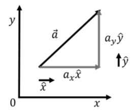
Now that we know how to add vectors, we can better understand the notation \(\vec a = a_x \hat x+ a_y\hat y\). This is not simply a notation, but is in fact algebraically correct. It means: “multiply the vector \(\hat x\) by \(a_x\) (thus giving it a length of \(a_x\)) and then add \(a_y\) times the vector \(\hat y\)”. This is illustrated in Figure A1.3.2, which shows the unit vectors, \(\hat x\) and \(\hat y\), which are then multiplied by \(a_x\) and \(a_y\), respectively, and then added together “head to tail”.

Figure A1.3.2: Illustration that the notation \(\vec a = a_{x}\hat x + a_{y}\hat y\) is in fact the vector addition of \(a_{x}\hat x\) and \(a_{y}\hat y\).

The scalar product

There are two ways to “multiply” vectors: the “scalar product” and the “vector product”. The scalar product (or “dot product”) takes two vectors and results in a scalar (a number). The vector product (or “cross product”) takes two vectors and results in a third vector.

The scalar product, \(\vec a \cdot \vec b\), of two vectors \(\vec a\) and \(\vec b\), is defined as the following:

\[\begin{aligned} \vec a \cdot \vec b=a_xb_x +a_yb_y\end{aligned}\]

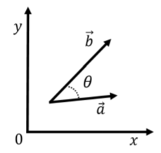
That is, one multiplies the individual components of the two vectors and then adds those products for each component. This is easily extended to the three dimensional case by adding a term \(a_zb_z\) to the sum. The scalar product is also related to the angle between the two vectors when the vectors are placed “tail to tail”, as in Figure A1.3.3

\[\begin{aligned} \vec a \cdot \vec b= ab\cos\theta\end{aligned}\]

Figure A1.3.3: Illustration of the angle between vectors \(\vec a\) and \(\vec b\) when these are placed tail to tail.

The scalar product between two vectors of a fixed length will be maximal when the two vectors are parallel (\(\cos\theta=1\)) and zero when the vectors are perpendicular (\(\cos\theta =0\)). The scalar product is thus useful when we want to calculate quantities that are maximal when two vectors are parallel.

Exercise \(\PageIndex{2}\)

The vectors \(\vec a\) and \(\vec b\) in the three diagrams below have the same magnitude. Order the diagrams from the one that gives the smallest scalar product \(\vec a\cdot \vec b\) to the largest scalar product.

Figure A1.3.4: Put these in order of the magnitude of their scalar product.

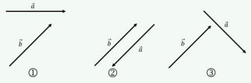
Answer

\(2<3<1\)

The vector product

The vector (or cross) product takes two vectors to produce a third vector that is mutually perpendicular to both vectors. The vector product only has meaning in three dimensions. Two vectors that are not co-linear, meaning they can not be arranged so that they lie along the same line, can always be used to define a plane in three dimensions. The cross product of those two vectors will give a third vector that is perpendicular to the plane (making it perpendicular to both vectors).

Algebraically, the three components of the vector product, \(\vec a\times \vec b\), of vectors \(\vec a\) and \(\vec b\) are found as follows:

\[ \vec a \times \vec b =\begin{pmatrix} a_yb_z - a_z b_y\\[4pt] a_zb_x - a_x b_z\\[4pt] a_xb_y - a_y b_x\\[4pt] \end{pmatrix}\]

One important property to note is that \(\vec a \times \vec b = -\vec b \times \vec a\); that is, the cross product is not commutative (the order matters). The magnitude of the vector obtained by a cross product is given by:

\[ ||\vec a \times \vec b ||=ab\sin\theta\]

where \(\theta\) is the angle between the vectors \(\vec a\) and \(\vec b\) when these are placed tail to tail (Figure A1.3.3). The vector resulting from a cross product will be null (have a zero length) if the vectors \(\vec a\) and \(\vec b\) are parallel, and will have a maximal length when these are perpendicular. The cross product is useful to determine quantities that are maximal when two vectors are perpendicular.

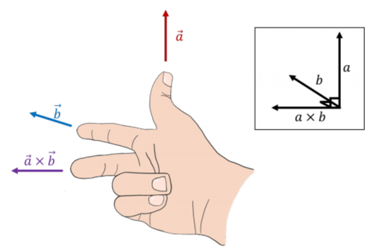
Geometrically, one can determine the direction of the cross product of two vectors by using a “right hand rule”. To distinguish it from another right hand rule (see Section A1.4), we will call it “the right hand rule for the cross product”). This is done by using your right hand, aligning your thumb with the first vector and your index with the second vector. The cross product will point in the direction of your middle finger (when you hold your middle finger perpendicular to the other two fingers). This is illustrated in Figure A1.3.5. Thus, you can often avoid using Equation A1.3.1 and instead use the right hand rule to determine the direction of the cross product and Equation A1.3.2 to find its magnitude.

Figure A1.3.5: Using the right hand rule for cross products to find the direction of the cross product of vectors \(\vec a\) (upwards) and \(\vec b\) (into the page).

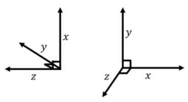
The unit vectors that define a coordinate system have the following properties relative to the cross product:

\[\begin{aligned} \vec x \times \vec y &= \vec z\\[4pt] \vec y \times \vec z &= \vec x\\[4pt] \vec z \times \vec x &= \vec y\\[4pt]\end{aligned}\]

For these properties to be correct, it should be noted that the direction of the \(z\) axis in three dimensions is specified by the choice of \(x\) and \(y\) axes. That is, one can freely choose the direction of the \(x\) and \(y\) axes, which then define a plane to which the \(z\) axis will be perpendicular. The direction of the \(z\) axis must be chosen so that \(\vec x \times \vec y = \vec z\) (this guarantees that the coordinate system is “right handed”), as in Figure A1.3.6.

Figure A1.3.6: Two possible orientations for a three dimensional coordinate system. You can confirm using the right hand rule that the \(z\) axis is the cross product \(\vec x × \vec y\).