25.4: Example uses of vectors in physics

This section gives a quick overview of some applications of vectors in physics.

Kinematics and vector equations

Kinematics is the description of the position and motion of an object (Chapters 3 and 4). The laws of physics are the principles that ultimately allow us to determine how the position of an object changes with time. For example, Newton’s Laws are a mathematical framework that introduce the concepts of force and mass in order to model and determine how an object will move through space.

We often use a position vector, \(\vec r(t)\), to describe the position of an object as a function of time. Because the object can move, the position vector is a function of time. A position vector is a special vector in the sense that it should be considered to be fixed in space; the position vector for an object points from the origin of a coordinate system to the location of the object.

The three components of the position vector in Cartesian coordinates, are the \(x\), \(y\), and \(z\) coordinates of the object:

\[\begin{aligned} \vec r(t) = \begin{pmatrix} x(t) \\[4pt] y(t) \\[4pt] z(t) \\[4pt] \end{pmatrix}\end{aligned}\]

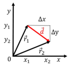
where the three coordinates of the object are functions of time if the object can move. Suppose that the object was initially at position \(\vec r_1=(x_1, y_1, z_1)\) at some time \(t=t_1\), and that later, at time \(t=t_2\), the object was at as second position, \(\vec r_2=(x_1, y_1, z_1)\). We can define the displacement vector, \(\vec d\), as the vector from position \(\vec r_1\) to position \(\vec r_2\):

\[\begin{aligned} \vec d = \vec r_2 - \vec r_1 =\begin{pmatrix} x_2-x_1 \\[4pt] y_2-y_1 \\[4pt] z_2-z_1 \\[4pt] \end{pmatrix} = \begin{pmatrix} \Delta x \\[4pt] \Delta y \\[4pt] \Delta z \\[4pt] \end{pmatrix}\end{aligned}\]

The displacement vector is such that one can add the vector \(\vec d\) to the vector \(\vec r_1\) to describe the new position of the object at time \(t_2\):

\[\begin{aligned} \vec d &= \vec r_2 - \vec r_1\\[4pt] \therefore \vec r_2 &= \vec r_1 + \vec d\end{aligned}\]

The components of the displacement vector, \(\Delta x\), \(\Delta y\), and \(\Delta z\) correspond to the displacements (the distance traveled) along the \(x\), \(y\), and \(z\) axes, respectively. This is illustrated for the two dimensional case in Figure A1.4.1.

Figure A1.4.1: Illustration of a displacement vector, \(\vec d = \vec r_{2} − \vec r_{1}\), for an object that was located at position \(\vec r_{1}\) at time \(t_{1}\) and at position \(\vec r_{2}\) at time \(t_{2}\).

The velocity vector of the object, \(\vec v=(v_x, v_y, v_z)\), is defined to be the displacement vector, \(\vec d\), divided by the amount of time (a scalar) that elapsed, \(\Delta t=t_2-t_1\), while the object moved by the corresponding displacement:

\[\begin{aligned} \vec v = \frac{\vec d}{\Delta t}=\begin{pmatrix} \frac{\Delta x}{\Delta t} \\[4pt] \frac{\Delta y}{\Delta t} \\[4pt] \frac{\Delta z}{\Delta t} \\[4pt] \end{pmatrix}\end{aligned}\]

We used the property that dividing a vector by a scalar (\(\Delta t\)) is defined as dividing each component by the scalar. If we write the components of the velocity vector out explicitly, we have:

\[\begin{aligned} \begin{pmatrix} v_x \\[4pt] v_y \\[4pt] v_z \\[4pt] \end{pmatrix} = \begin{pmatrix} \frac{\Delta x}{\Delta t} \\[4pt] \frac{\Delta y}{\Delta t} \\[4pt] \frac{\Delta z}{\Delta t} \end{pmatrix}\end{aligned}\]

That is, we can think of each row in this “vector equation” as an independent equation. That is, when we write the vector equation:

\[\begin{aligned} \vec v = \frac{\vec d}{\Delta t}\end{aligned}\]

we are really just using a shorthand notation for writing the three independent equations that are true for each individual component of the vectors:

\[\begin{aligned} v_x &= \frac{\Delta x}{\Delta t} \\[4pt] v_y &= \frac{\Delta y}{\Delta t} \\[4pt] v_z &= \frac{\Delta z}{\Delta t} \\[4pt]\end{aligned}\]

Whenever we write an equation using vectors, we are really writing out multiple equations all at once, one for each component. Newton’s Second Law:

\[\begin{aligned} \vec F = m \vec a\end{aligned}\]

thus corresponds to the three (scalar) equations:

\[\begin{aligned} F_x &= ma_x\\[4pt] F_y &= ma_y\\[4pt] F_z &= ma_z\\[4pt]\end{aligned}\]

Work and scalar products

As we will see, “work” is a scalar quantity that allows us to determine the change in the speed (squared) of an object that results from a force exerted over a particular displacement (Chapter 7). Both force and the displacement are vector quantities (a force has a magnitude and is exerted in a particular direction). The work, \(W\), done by a force, \(\vec F\), over a displacements, \(\vec d\), is defined as:

\[\begin{aligned} W = \vec F \cdot \vec d\end{aligned}\]

The work energy theorem tells us that this work is related to the change in speed squared of the object as it moves along the displacement vector \(d\). If the work is zero, the object has the same speed at the beginning and end of the displacement. If the work is positive, the object is moving faster at the end of the displacement (and slower if the work is negative). A one dimensional example is shown in Figure A1.4.2, which shows a force \(\vec F\) being applied to a block as it slides along the ground over a distance \(d\) (represented by the displacement vector \(\vec d\)).

Figure A1.4.2: Example of a force \(\vec F\) being applied on an object as it moves along the displacement vector \(\vec d\).

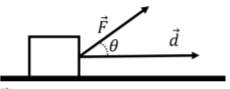
Intuitively, it makes sense that only the horizontal component of the force would contribute to changing the speed of the object as it moves along the horizontal trajectory defined by the vector \(\vec d\). The vertical component of the force does not contribute to changing the speed of the object. Thus, the work (the change in speed), should only depend on the component of the force that is parallel to the displacement vector. The scalar product allows us to formalize this in an equation. The scalar product is given by:

\[\begin{aligned} \vec F \cdot \vec d = Fd\cos\theta = F_{\parallel}d\end{aligned}\]

where we introduced \(F_{\parallel} = F\cos\theta\) as the component of \(\vec F\) that is parallel to \(\vec d\) (see Figure A1.4.2). The scalar product thus “picks out” the component of \(\vec F\) that is parallel to \(\vec d\), which is exactly what we need to in order for work to make sense.

Using vectors to describe rotational motion

Often, we need to describe rotational motion in physics. If an object is rotating, one must specify:

1. The axis about which the object is rotating
2. The direction about that axis in which the object is rotating (e.g. clockwise or counter-clockwise)
3. How fast the object is rotating

We introduce a new type of vector, an “axial vector”, to describe this kind of rotational motion. We choose the direction of the vector to be co-linear with the axis of rotation and the magnitude of the vector to represent the speed with which the object is rotating. We are thus left with two choices for the direction of the vector. For example, consider the wheels on a car that is moving away from you (Figure A1.4.3, the car is moving into the page). The axis of rotation is the axis of the wheel, so we know that the vector describing the wheel’s rotation (the angular velocity vector) must point either to the left or to the right.

Figure A1.4.3: The wheels on a car that is driving away from you.

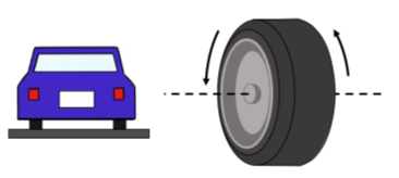
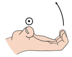
We choose the direction of the vector by using another right hand rule. We will refer to this as “the right hand rule for axial vectors” to distinguish it from the right hand rule for the cross product. When using the right hand rule for axial vectors, the vector points in the direction of your thumb when you curl your fingers in the direction of rotation, as in Figure A1.4.4. For the car moving away from you, the wheels will be turning such that the closest point to you is moving up and the furthest point is moving down. Using the right hand rule, we find that the rotation vector points to the left.

Figure A1.4.4: Using the right hand rule for axial quantities. In this case, the direction of rotation is counter clockwise when looking at the page (the direction that the fingers curl), so the rotation vector points out of the page (the direction of the thumb).

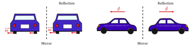
We have to distinguish axial vectors from “true” vectors because they do not behave like true vectors in all cases. For instance, imagine that there is a giant mirror that runs parallel to the road (Figure A1.4.5). When the car is reflected in the mirror, the reflected car will also be moving away from you. This means that the wheels will be turning in the same direction as before, so the rotation vector still points to the left. Now consider a true vector, like a velocity vector. If the velocity vector initially pointed to the left (i.e. if the car was moving to the left), the reflected car would be moving to the right. So, we expect a true vector to change directions when it is reflected in this way. Since the rotation vector does not always behave like a true vector, we call it an axial vector or a “pseudovector.”

Figure A1.4.5: Left: The angular velocity vector for the rotation of the wheels, \(\vec ω\), which points to the left, also points left in the reflection. Right: The velocity vector, pointing to the left, points to the right in the reflection of the car. The angular velocity vector is called an “axial” or “pseudo” vector because it does not change direction under a reflection.

Torque and vector products

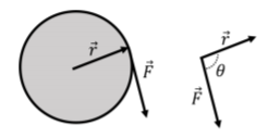
We will introduce the concept of a torque in order to describe how a force can cause an object to rotate. Consider the disk illustrated in Figure A1.4.6 that is free to rotate about an axis that goes through its center and that is perpendicular to the plane of the page. A force \(\vec F\) is applied at the edge of the disk (imagine pulling on a string attached to the edge of the disk), at a position that is displaced from the axis of rotation by the vector \(\vec r\). The torque, \(\vec \tau\), of the force about the center of the disk is defined to be:

\[\begin{aligned} \vec\tau=\vec r\times \vec F\end{aligned}\]

and represents how much the force \(\vec F\) will contribute to making the disk rotate about its axis. If the force vector were parallel to the vector \(\vec r\), the disk would not rotate; if you pull outwards on a disk, it will not rotate about its center. However, if the force is perpendicular to the vector \(\vec r\) (i.e. tangent to the circumference of the disk), then it will maximally cause the disk to rotate. The magnitude of the torque (cross-product) is given by:

\[\begin{aligned} \tau =rF\sin\theta=F_{\perp}r=Fr_\perp\end{aligned}\]

where \(\theta\) is the angle between the vectors when placed tail to tail, as in the right side of Figure A1.4.6. In the last two equalities, we have defined \(F_\perp=F\sin\theta\) or \(r_\perp=r\sin\theta\) to refer to the part of the vector \(\vec F\) that is perpendicular to the vector \(\vec r\) or the part of the vector \(\vec r\) that is perpendicular to the vector \(\vec F\). That is, the vector product “picks out” the part of a vector that is perpendicular to the other, which is exactly the property that we need for the physical quantity of torque.

Figure A1.4.6: A force, \(\vec F\), is exerted in the plane of a disk at a position given by the vector \(\vec r\) relative to the center of the disk.

Exercise \(\PageIndex{1}\)

Referring to Figure A1.4.6, in which direction does the torque vector point?

1. to the right
2. to the left
3. out of the page
4. into the page

Answer