
16.A: Math
- Page ID
- 17466

\( \newcommand{\vecs}[1]{\overset { \scriptstyle \rightharpoonup} {\mathbf{#1}} } \)
\( \newcommand{\vecd}[1]{\overset{-\!-\!\rightharpoonup}{\vphantom{a}\smash {#1}}} \)
\( \newcommand{\dsum}{\displaystyle\sum\limits} \)
\( \newcommand{\dint}{\displaystyle\int\limits} \)
\( \newcommand{\dlim}{\displaystyle\lim\limits} \)
\( \newcommand{\id}{\mathrm{id}}\) \( \newcommand{\Span}{\mathrm{span}}\)
( \newcommand{\kernel}{\mathrm{null}\,}\) \( \newcommand{\range}{\mathrm{range}\,}\)
\( \newcommand{\RealPart}{\mathrm{Re}}\) \( \newcommand{\ImaginaryPart}{\mathrm{Im}}\)
\( \newcommand{\Argument}{\mathrm{Arg}}\) \( \newcommand{\norm}[1]{\| #1 \|}\)
\( \newcommand{\inner}[2]{\langle #1, #2 \rangle}\)
\( \newcommand{\Span}{\mathrm{span}}\)
\( \newcommand{\id}{\mathrm{id}}\)
\( \newcommand{\Span}{\mathrm{span}}\)
\( \newcommand{\kernel}{\mathrm{null}\,}\)
\( \newcommand{\range}{\mathrm{range}\,}\)
\( \newcommand{\RealPart}{\mathrm{Re}}\)
\( \newcommand{\ImaginaryPart}{\mathrm{Im}}\)
\( \newcommand{\Argument}{\mathrm{Arg}}\)
\( \newcommand{\norm}[1]{\| #1 \|}\)
\( \newcommand{\inner}[2]{\langle #1, #2 \rangle}\)
\( \newcommand{\Span}{\mathrm{span}}\) \( \newcommand{\AA}{\unicode[.8,0]{x212B}}\)
\( \newcommand{\vectorA}[1]{\vec{#1}} % arrow\)
\( \newcommand{\vectorAt}[1]{\vec{\text{#1}}} % arrow\)
\( \newcommand{\vectorB}[1]{\overset { \scriptstyle \rightharpoonup} {\mathbf{#1}} } \)
\( \newcommand{\vectorC}[1]{\textbf{#1}} \)
\( \newcommand{\vectorD}[1]{\overrightarrow{#1}} \)
\( \newcommand{\vectorDt}[1]{\overrightarrow{\text{#1}}} \)
\( \newcommand{\vectE}[1]{\overset{-\!-\!\rightharpoonup}{\vphantom{a}\smash{\mathbf {#1}}}} \)
\( \newcommand{\vecs}[1]{\overset { \scriptstyle \rightharpoonup} {\mathbf{#1}} } \)
\(\newcommand{\longvect}{\overrightarrow}\)
\( \newcommand{\vecd}[1]{\overset{-\!-\!\rightharpoonup}{\vphantom{a}\smash {#1}}} \)
\(\newcommand{\avec}{\mathbf a}\) \(\newcommand{\bvec}{\mathbf b}\) \(\newcommand{\cvec}{\mathbf c}\) \(\newcommand{\dvec}{\mathbf d}\) \(\newcommand{\dtil}{\widetilde{\mathbf d}}\) \(\newcommand{\evec}{\mathbf e}\) \(\newcommand{\fvec}{\mathbf f}\) \(\newcommand{\nvec}{\mathbf n}\) \(\newcommand{\pvec}{\mathbf p}\) \(\newcommand{\qvec}{\mathbf q}\) \(\newcommand{\svec}{\mathbf s}\) \(\newcommand{\tvec}{\mathbf t}\) \(\newcommand{\uvec}{\mathbf u}\) \(\newcommand{\vvec}{\mathbf v}\) \(\newcommand{\wvec}{\mathbf w}\) \(\newcommand{\xvec}{\mathbf x}\) \(\newcommand{\yvec}{\mathbf y}\) \(\newcommand{\zvec}{\mathbf z}\) \(\newcommand{\rvec}{\mathbf r}\) \(\newcommand{\mvec}{\mathbf m}\) \(\newcommand{\zerovec}{\mathbf 0}\) \(\newcommand{\onevec}{\mathbf 1}\) \(\newcommand{\real}{\mathbb R}\) \(\newcommand{\twovec}[2]{\left[\begin{array}{r}#1 \\ #2 \end{array}\right]}\) \(\newcommand{\ctwovec}[2]{\left[\begin{array}{c}#1 \\ #2 \end{array}\right]}\) \(\newcommand{\threevec}[3]{\left[\begin{array}{r}#1 \\ #2 \\ #3 \end{array}\right]}\) \(\newcommand{\cthreevec}[3]{\left[\begin{array}{c}#1 \\ #2 \\ #3 \end{array}\right]}\) \(\newcommand{\fourvec}[4]{\left[\begin{array}{r}#1 \\ #2 \\ #3 \\ #4 \end{array}\right]}\) \(\newcommand{\cfourvec}[4]{\left[\begin{array}{c}#1 \\ #2 \\ #3 \\ #4 \end{array}\right]}\) \(\newcommand{\fivevec}[5]{\left[\begin{array}{r}#1 \\ #2 \\ #3 \\ #4 \\ #5 \\ \end{array}\right]}\) \(\newcommand{\cfivevec}[5]{\left[\begin{array}{c}#1 \\ #2 \\ #3 \\ #4 \\ #5 \\ \end{array}\right]}\) \(\newcommand{\mattwo}[4]{\left[\begin{array}{rr}#1 \amp #2 \\ #3 \amp #4 \\ \end{array}\right]}\) \(\newcommand{\laspan}[1]{\text{Span}\{#1\}}\) \(\newcommand{\bcal}{\cal B}\) \(\newcommand{\ccal}{\cal C}\) \(\newcommand{\scal}{\cal S}\) \(\newcommand{\wcal}{\cal W}\) \(\newcommand{\ecal}{\cal E}\) \(\newcommand{\coords}[2]{\left\{#1\right\}_{#2}}\) \(\newcommand{\gray}[1]{\color{gray}{#1}}\) \(\newcommand{\lgray}[1]{\color{lightgray}{#1}}\) \(\newcommand{\rank}{\operatorname{rank}}\) \(\newcommand{\row}{\text{Row}}\) \(\newcommand{\col}{\text{Col}}\) \(\renewcommand{\row}{\text{Row}}\) \(\newcommand{\nul}{\text{Nul}}\) \(\newcommand{\var}{\text{Var}}\) \(\newcommand{\corr}{\text{corr}}\) \(\newcommand{\len}[1]{\left|#1\right|}\) \(\newcommand{\bbar}{\overline{\bvec}}\) \(\newcommand{\bhat}{\widehat{\bvec}}\) \(\newcommand{\bperp}{\bvec^\perp}\) \(\newcommand{\xhat}{\widehat{\xvec}}\) \(\newcommand{\vhat}{\widehat{\vvec}}\) \(\newcommand{\uhat}{\widehat{\uvec}}\) \(\newcommand{\what}{\widehat{\wvec}}\) \(\newcommand{\Sighat}{\widehat{\Sigma}}\) \(\newcommand{\lt}{<}\) \(\newcommand{\gt}{>}\) \(\newcommand{\amp}{&}\) \(\definecolor{fillinmathshade}{gray}{0.9}\)Vector Basics
Classical mechanics describes the motion of bodies as they move through space. To describe a motion in space it is not sufficient to give a position and a speed: you need a direction as well. Therefore we work with vectors: mathematical objects that have both a magnitude and a direction. If you tell me you’re moving, I know something, but not much; I’ll know more if you tell me you’re moving at walking speed, and have full information of your velocity once you tell me that you’re moving at walking speed towards the coffee machine. Although in principle we could make do with specifying a magnitude and direction of every vector in this way, it is often more convenient to express our vectors in a basis. To do so, we choose an (arbitrary) origin, and as many basis vectors as we have spatial dimensions, in such a way that they are not parallel to one another, and usually mutually perpendicular (orthogonal) and of unit length (orthonormal). Then we decompose our vector by giving its components along each of the basis vectors. The most common choice is to use a Cartesian basis, of two or three (depending on spatial dimension) basis vectors of unit length pointing in the standard x, y and z directions, and indicated as \(\hat{\boldsymbol{x}}, \hat{\boldsymbol{y}}\) and \(\hat{\boldsymbol{z}}\), or (rather annoyingly) sometimes as \(\boldsymbol{i}, \boldsymbol{j}\) and \(\boldsymbol{k}\), the latter especially in American textbooks. Other often encountered systems are polar coordinates (2D) and cylindrical and spherical coordinates (3D), see the mathematical appendix for more background on those. To write our vectors, we now specify the components in each direction, writing for example \(\boldsymbol{v}=3 \hat{\boldsymbol{x}}+3 \hat{\boldsymbol{y}}\) for a vector (in boldface) representing a speed of \(3 \sqrt{2}\) and a direction making an angle of \(45^{\circ}\) with the horizontal.
Vectors can be added and subtracted just like scalars - simply add and subtract them by component. Graphically, you add two vectors by putting them head-to-tail: you can find the sum of two vectors \(\boldsymbol{v}\) and \(\boldsymbol{w}\) by putting the start of \(\boldsymbol{w}\) at the end of \(\boldsymbol{v}\), the sum \(\boldsymbol{v} + \boldsymbol{w}\) then points from the start of \(\boldsymbol{v}\) to the end of \(\boldsymbol{w}\). You can also multiply a vector by a scalar, by multiplying every component of the vector with that scalar. Graphically, this means that you extend the length of the vector with the scalar factor you just multiplied with.
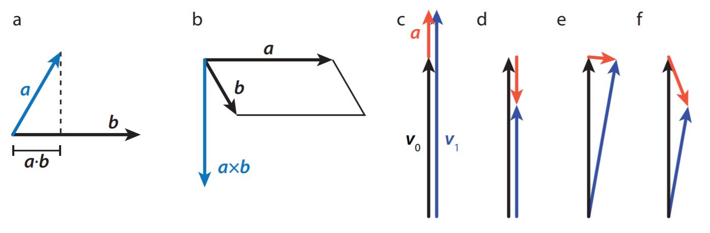
You can’t take the product of two vectors like you would two scalars. There are however two vector operations that closely resemble the product, known as the inner (or dot) and outer (or cross) product, see Figure 16.A.1. The dot product represents the length of the projection of one vector on another (and thus gives a scalar); it is zero for perpendicular vectors, and the dot product of a vector with itself gives the square of its length. To calculate the dot product of two vectors, sum the products of their components: if \(\boldsymbol{v}=v_{x} \hat{\boldsymbol{x}}+v_{y} \hat{\boldsymbol{y}}\) and \(\boldsymbol{w}=w_{x} \hat{\boldsymbol{x}}+w_{y} \hat{y}\), then \(\boldsymbol{v} \cdot \boldsymbol{w}=v_{x} w_{x}+v_{y} w_{y}\). You can use the dot product to find the angle between two vectors, using standard geometry, which gives
\[\cos \theta=\frac{\boldsymbol{v} \cdot \boldsymbol{w}}{|\boldsymbol{v}||\boldsymbol{w}|}=\frac{v_{x} w_{x}+v_{y} w_{y}}{|\boldsymbol{v}||\boldsymbol{w}|}\]
where \(|\boldsymbol{v}|\) and \(|\boldsymbol{w}|\) are the lengths of vectors \(\boldsymbol{v}\) and \(\boldsymbol{w}\), respectively. The cross product is only defined for three-dimensional vectors, say \(\boldsymbol{v}=v_{x} \hat{\boldsymbol{x}}+v_{y} \hat{\boldsymbol{y}}+v_{z} \hat{\boldsymbol{z}}\) and \(\boldsymbol{w}=w_{x} \hat{\boldsymbol{x}}+w_{y} \hat{\boldsymbol{y}}+w_{z} \hat{z}\). The result is another vector, with a direction perpendicular to the plane spanned by \(\boldsymbol{v}\) and \(\boldsymbol{w}\), and a magnitude equal to the area of the parallelogram bounded by them. The cross product is most easily expressed in column vector form:
\[\boldsymbol{v} \times \boldsymbol{w}=\left(\begin{array}{c}
{v_{x}} \\
{v_{y}} \\
{v_{z}}
\end{array}\right) \times\left(\begin{array}{c}
{w_{x}} \\
{w_{y}} \\
{w_{z}}
\end{array}\right)=\left(\begin{array}{c}
{v_{y} w_{z}-v_{z} w_{y}} \\
{v_{z} w_{x}-v_{x} w_{z}} \\
{v_{x} w_{y}-v_{y} w_{x}}
\end{array}\right)\]
The cross product of a vector with itself is zero.
Vectors can be functions, just like scalar quantities: they can depend on one or more parameters, like position or time. Also, again just like scalar functions, you can calculate a rate of change of vector function as you move through parameter values, for instance asking how the velocity of a car changes as a function of time. An instantaneous rate of change is simply a derivative, which is calculated in exactly the same manner as the derivative of a scalar function. For example, the rate of change of the velocity, known as the acceleration \(\boldsymbol{a}\), is defined as:
\[\boldsymbol{a}=\lim _{\Delta t \rightarrow 0} \frac{\boldsymbol{v}(t+\Delta t)-\boldsymbol{v}}{\Delta t}\]
Since the velocity itself is the derivative of the position \(\boldsymbol{x}(t)\), the acceleration is also the second derivative of the position. Time derivatives occur so frequently in classical mechanics that we use a special notation for them: a first derivative is indicated by a dot on top of the quantity, and a second derivative by a double dot - so we have \(\boldsymbol{a}=\boldsymbol{\dot { x }}=\ddot{\boldsymbol{x}}\).
Vector derivatives are somewhat richer than those of scalar functions, since there are more ways that a vector can change. Like a scalar function, the magnitude of a vector can increase or decrease. Moreover, its direction can also change, which also means that it has a nonzero derivative, and of course, you can have a combination of a change in magnitude and a change in direction, see Figure 16.A.1.
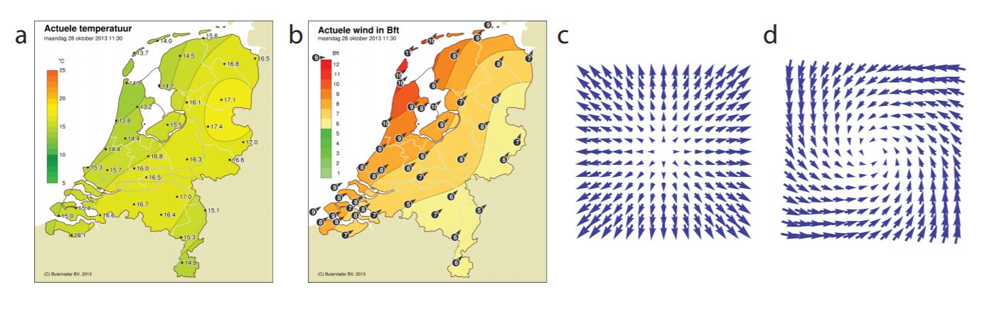
Functions (scalar or vector) that are defined at every point in space are sometimes called fields. Examples are the temperature (scalar) and wind (vector) at every point on the planet, see Figure 16.A.2. Just like you can calculate the rate of change of a function in time, you can also consider how a function changes in space. For a scalar function, this quantity is a vector, known as the gradient, defined as the vector of partial derivatives. For a function f (x, y, z), we have:
\[\boldsymbol{\nabla} f=\frac{\partial f}{\partial x} \hat{\boldsymbol{x}}+\frac{\partial f}{\partial y} \hat{\boldsymbol{y}}+\frac{\partial f}{\partial z} \hat{\boldsymbol{z}}=\left(\begin{array}{c}
{\partial f / \partial x} \\
{\partial f / \partial y} \\
{\partial f / \partial z}
\end{array}\right)\]
The direction of \(\boldsymbol{\nabla} f\) is the direction of maximal change, and its magnitude tells you how quickly the function changes in that direction. For a vector field \(\boldsymbol{v}\), we can’t take the gradient, but we can use the ‘vector’ \(\boldsymbol{\nabla}\) of partial derivatives combined with either the dot or cross product. The first option is known as the divergence of \(\boldsymbol{v}\), and tells you how quickly \(\boldsymbol{v}\) spreads out; the second is the curl of \(\boldsymbol{v}\) and tells you how much \(\boldsymbol{v}\) rotates:
\[\begin{align}
\operatorname{div}(\boldsymbol{v}) &=\boldsymbol{\nabla} \cdot \boldsymbol{v}=\frac{\partial v_{x}}{\partial x}+\frac{\partial v_{y}}{\partial y}+\frac{\partial v_{z}}{\partial z} \\
\operatorname{curl}(\boldsymbol{v}) &=\boldsymbol{\nabla} \times \boldsymbol{v}=\left(\begin{array}{c}
{\partial_{y} v_{z}-\partial_{z} v_{y}} \\
{\partial_{z} v_{x}-\partial_{x} v_{z}} \\
{\partial_{x} v_{y}-\partial_{y} v_{x}}
\end{array}\right)
\end{align}\]
where \(\partial_{x}= \frac{\partial}{\partial x}\), and so on.
Polar Coordinates
You can specify any point in the plane by specifying its projection on two perpendicular axes - we typically call these the x and y-axes and x and y coordinates. In this Cartesian system (named after Descartes), we identify unit vectors \(\hat{\boldsymbol{x}}\) and \(\hat{\boldsymbol{y}}\), pointing along their respective axes, and being of unit length. A position \(\boldsymbol{r}\) can then be decomposed in the two directions: \(\boldsymbol{r}=r_{x} \hat{\boldsymbol{x}}+r_{y} \hat{\boldsymbol{y}}\), with \(r_{x}=\boldsymbol{r} \cdot \hat{\boldsymbol{x}}\) and \(r_{y}=\boldsymbol{r} \cdot \hat{\boldsymbol{y}}\). Alternatively, we can write \(\hat{\boldsymbol{x}}=\left(\begin{array}{l}
{1} \\
{0}
\end{array}\right)\) and \(\hat{\boldsymbol{y}}=\left(\begin{array}{l}
{0} \\
{1}
\end{array}\right)\), which gives for \(\boldsymbol{r}\):
\[\boldsymbol{r}=r_{x} \hat{\boldsymbol{x}}+r_{y} \hat{\boldsymbol{y}}=\left(\begin{array}{l}
{r_{x}} \\
{r_{y}}
\end{array}\right)\]
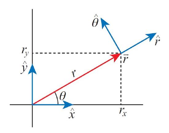
Instead of specifying the x and y coordinates of our position, we could also uniquely identify it by giving two different numbers: its distance to the origin r, and the angle \(\theta\) the line to the origin makes with a fixed reference axis (typically the x-axis), see Figure 16.A.3. Invoking the Pythagorean theorem and basic trigonometry,
we readily find \(r=\sqrt{r_{x}^{2}+r_{y}^{2}}\) and \(\tan \theta= \frac{r_{y}}{r_{x}}\). We call r the length of the vector \(\boldsymbol{r}\). We could also invert the relations for r and \(\theta\) so we can get the Cartesian components if the length and angle are known: \(r_{x}=r \cos \theta\) and \(r_{y}=r \sin \theta\).
Like the Cartesian basis vectors \(\hat{\boldsymbol{x}}\) and (\hat{\boldsymbol{y}}\), which point in the direction of increasing x and y values, we can also define unit vectors pointing in the direction of increasing r and \(\theta\). These directions do depend on our position in space, but they do have a clear geometrical interpretation: \hat{\boldsymbol{r}} always points radially outward from the origin, and \hat{\boldsymbol{\theta}} in the direction you’d move if you’d be making a counterclockwise rotation about the origin. Given a position vector \(\boldsymbol{r}\), finding the vector in the direction of increasing r is very easy: \(\hat{\boldsymbol{r}}= \boldsymbol{r} / r\). The expression for r in our new polar basis \((\hat{\boldsymbol{r}}, \hat{\boldsymbol{\theta}})\) is almost tautological: \(\boldsymbol{r}=r \hat{\boldsymbol{r}}\).
Relating the polar basis vectors to the Cartesian ones is straightforward. We have:
\[\boldsymbol{r}=r_{x} \hat{\boldsymbol{x}}+r_{y} \hat{\boldsymbol{y}}=r \hat{\boldsymbol{r}}\]
and using \(r_{x}=r \cos \theta, r_{y}=r \sin \theta\) we also have
\[\boldsymbol{r}=r \cos \theta \hat{\boldsymbol{x}}+r \sin \theta \hat{\boldsymbol{y}}\]
We thus find that \(\hat{\boldsymbol{r}}=\cos \theta \hat{\boldsymbol{x}}+\sin \theta \hat{\boldsymbol{y}}\).
For \(\hat{\boldsymbol{\theta}\) we note that to rotate around the origin, the direction of motion needs to be perpendicular to \(\hat{\boldsymbol{r}}\). There are of course two such directions - we pick the sign by demanding that the counterclockwise rotation is positive. This gives \(\hat{\boldsymbol{\theta}}=\left(r_{y} / r\right) \hat{\boldsymbol{x}}-\left(r_{x} / r\right) \hat{\boldsymbol{y}}=\sin \theta \hat{\boldsymbol{x}}-\cos \theta \hat{\boldsymbol{y}}\). Written out as vectors, we have:
\[\hat{\boldsymbol{r}}=\left(\begin{array}{c}
{\cos \theta} \\
{\sin \theta}
\end{array}\right), \quad \hat{\boldsymbol{\theta}}=\left(\begin{array}{c}
{\sin \theta} \\
{-\cos \theta}
\end{array}\right)\]
Note that
\[\hat{\boldsymbol{r}}=\frac{\partial \hat{\boldsymbol{\theta}}}{\partial \theta}, \quad \hat{\boldsymbol{\theta}}=-\frac{\partial \hat{\boldsymbol{r}}}{\partial \theta}\]
Naturally, we can also express the Cartesian basis in terms of the polar ones:
\[\hat{\boldsymbol{x}}=\cos \theta \hat{\boldsymbol{r}}+\sin \theta \hat{\boldsymbol{\theta}}, \quad \hat{\boldsymbol{y}}=\sin \theta \hat{\boldsymbol{r}}-\cos \theta \hat{\boldsymbol{\theta}}\]
Solving Differential Equations
A differential equation is an equation which contains derivatives of the function to be determined. They can be very simple. For example, you may be given the (constant) velocity of a car, which is the derivative of its position, which we’d write mathematically as:
\[v=\frac{\mathrm{d} x}{\mathrm{d} t}=v_{0} \label{velocity}\]
To determine where the car ends up after one hour, we need to solve this differential equation. We also need a second piece of information: where the car was at some reference time (usually t = 0), the initial condition. If \(x(0) = 0\), you don’t need advanced maths skills to figure out that \(x(1 hour) = v0 \cdot (1 hour)\). Unfortunately, things aren’t usually this easy.
Before we proceed to a few techniques for solving differential equations, we need some terminology. The order of a differential equation is the order of the highest derivative found in the equation; Equation \ref{velocity} is thus of first order. A differential equation is called ordinary if it only contains derivatives with respect to one variable, and partial if it contains derivatives to multiple variables. The equation is linear if it does not contain any products of (derivatives of) the unknown function. Finally, a differential equation is homogeneous if it only contains terms that contain the unknown function, and inhomogeneous if it also contains other terms. Equation \ref{velocity} is ordinary and inhomogeneous, as the \(v_0\) term on the right does not contain the unknown function \(x(t )\). In the sections below,we discuss the various cases you’ll encounter in this book; there are many others (many of which can’t be solved explicitly) to which a whole subfield of mathematics is dedicated.
A.3.1. FIRST-ORDER LINEAR ORDINARY DIFFERENTIAL EQUATIONS
Suppose we have a general equation of the form
\[a(t) \frac{\mathrm{d} x}{\mathrm{d} t}+b(t) x(t)=f(t) \label{A.11}\]
where \(a(t ), b(t )\) and \(f (t )\) are known functions of \(t \), and \(x(t )\) is our unknown function. Equation \ref{A.11} is a first-order, ordinary, linear, inhomogeneous differential equation. In order to solve it we will use two techniques that are tremendously useful: separation of variables and separation into homogeneous and particular solutions.
Suppose we had \(f (t ) = 0\). Then, if we had two solutions \(x_1 (t )\) and \(x_2 (t )\) of Equation \ref{A.11}, we could construct a third as \(x_{1}(t)+x_{2}(t)\) (or any linear combination of \(x_1 (t )\) and \(x_2 (t )\) ), since the equation is linear. Now since \(f (t )\) is not zero, we can’t do this, but we can do something else. First, we find the most general solution to the equation where \(f (t ) = 0\), which we call the homogeneous solution \(x_h (t )\). Second, we find a solution (any at all) of the full Equation \ref{A.11}, which we call the particular solution \(x_p (t )\). The full solution is then the sum of these two solutions, \(x(t)=x_{\mathrm{h}}(t)+x_{\mathrm{p}}(t)\). You may worry that there may be multiple particular solutions: how would we pick the ‘right’ one? Fortunately, we don’t need to worry: the homogeneous solution will contain an unknown variable, which will be set by the initial condition. Changing the particular solution will change the value of the variable, such that the final solution will be the same and satisfy both the differential equation and the initial condition.
To find the solution to the homogeneous equation
\[a(t) \frac{\mathrm{d} x_{\mathrm{h}}}{\mathrm{d} t}+b(t) x_{\mathrm{h}}(t)=0 \label{A.12}\]
we’re going to use a technique called separation of variables. There are two variables in this system: the independent parameter t and the dependent parameter x. The trick is to get everything depending on t on one side of the equals sign, and everything depending on x on the other. To do so, we’re going to treat dx/dt as if it were an actual fraction1. In that case, it’s not hard to see that we can re-arrange Equation \ref{A.12} to
\[\frac{1}{x_{\mathrm{h}}} \mathrm{d} x_{\mathrm{h}}=-\frac{b(t)}{a(t)} \mathrm{d} t \label{A.13}\]
By itself, Equation \ref{A.13} means little, but if we integrate both sides, we get something that makes sense:
\[\int \frac{1}{x_{\mathrm{h}}} \mathrm{d} x_{\mathrm{h}}=\log \left(x_{\mathrm{h}}\right)+C=-\int \frac{b(t)}{a(t)} \mathrm{d} t\]
or
\[x_{\mathrm{h}}(t)=A \exp \left[-\int \frac{b(t)}{a(t)} \mathrm{d} t\right] \label{A.15}\]
where \(A = exp(C)\) is an integration constant (the unknown constant that will be set by our initial condition). Of course, in principle it may not be possible to evaluate the integral in Equation \ref{A.15}, but even then the solution is valid. In practice, you’ll often encounter situations in which \(a(t )\) and \(b(t )\) are simple functions or even constants, and the evaluation of the integral is straightforward. Now that we have our homogeneous solution, we still need a particular one. Sometimes you’re lucky, and you can easily guess one - for instance one in which \(x_p (t )\) doesn’t depend on \(t\) at all. In case you’re not lucky, there’s are two other techniques you may try, either using variation of constants or finding an integrating factor. To demonstrate variation of constants, we’ll pick a specific example, to not get lost in a bunch of abstract functions. Let \(a(t ) = a\) be a constant and \(b(t ) = bt\) be linear. The homogeneous solution then becomes \(x_{\mathrm{h}}(t)=A \exp \left[-\frac{1}{2} \frac{b}{a} t^{2}\right]\). The constant we’re going to vary is our integration constant \(A\), so our guess for the particular solution will be
\[x_{\mathrm{p}}(t)=A(t) \exp \left[-\frac{1}{2} \frac{b}{a} t^{2}\right] \label{A.16}\]
We substitute \ref{A.16} back into the full differential Equation \ref{A.11}, which gives:
\[\left[a \frac{\mathrm{d} A}{\mathrm{d} t}-a A(t) \frac{b t}{a}+b t A(t)\right] \exp \left[-\frac{1}{2} \frac{b}{a} t^{2}\right]=a \frac{\mathrm{d} A}{\mathrm{d} t} \exp \left[-\frac{1}{2} \frac{b}{a} t^{2}\right]=f(t)\]
A big part of the left-hand side thus cancels, and that’s not a coincidence - that’s because it is based on the homogeneous equation. What remains is a differential equation in \(A(t )\) that can be trivially solved by direct integration:
\[A(t)=\int \frac{\mathrm{d} A}{\mathrm{d} t} \mathrm{d} t=\frac{1}{a} \int f(t) \exp \left[\frac{1}{2} \frac{b}{a} t^{2}\right] \mathrm{d} t \label{A.18}\]
Again, it may not be possible to evaluate the integral in Equation \ref{A.18}, but in principle the solution could be inserted in Equation \ref{A.16} to give us our particular solution, and the whole differential equation will be solved.
Alternatively, we may try to find an integration factor for Equation \ref{A.11}. This means that we try to rewrite the left hand side of the equation as a total derivative, after which we can simply integrate to get the solution. To do so, we first divide the whole equation by \(a(t )\), then look for a function \(\mu (t )\) that satisfies the condition that
\[\frac{\mathrm{d}}{\mathrm{d} t}[\mu(t) x(t)]=\mu(t) \frac{\mathrm{d} x}{\mathrm{d} t}+x(t) \frac{\mathrm{d} \mu}{\mathrm{d} t} \bmod e l s \mu(t) \frac{\mathrm{d} x}{\mathrm{d} t}+\mu(t) \frac{b(t)}{a(t)} x(t)\]
from which we can read off that we need to solve the homogeneous equation
\[\frac{\mathrm{d} \mu}{\mathrm{d} t}=\frac{b(t)}{a(t)} \mu(t) \label{A.20}\]
We can solve \ref{A.20} by separation of constants, which gives us
\[\mu(t)=\exp \left(\int \frac{b(t)}{a(t)} \mathrm{d} t\right)\]
where we set the integration constant to one, as it drops out of the equation for \(x(t )\) anyway. With this function \(\mu (t )\), we can rewrite Equation \ref{A.11} as
\[\frac{\mathrm{d}}{\mathrm{d} t}[\mu(t) x(t)]=\mu(t) \frac{f(t)}{a(t)}\]
which we can integrate to find \(x(t )\):
\[x(t)=\frac{1}{\mu(t)} \int \mu(t) \frac{f(t)}{a(t)} \mathrm{d} t\]
A.3.2. SECOND-ORDER LINEAR ORDINARY DIFFERENTIAL EQUATIONS WITH CONSTANT COEFFICIENTS
Second order ordinary differential equations are essential for the study of mechanics, as its central equation, Newton’s second law of motion (Equation 2.1.4) is of this type. In the case that the equation is also linear, we have some hopes of solving it analytically. There are several examples of this type of equation in the main text, especially in Section 2.6, where we solve the equation of motion resulting from Newton’s second law for three special cases, and Section 8.1, where we study a number of variants of the harmonic oscillator. For the case that the equation is homogeneous and has constant coefficients, we can write down the general solution2. The equation to be solved is of the form
\[a \frac{\mathrm{d}^{2} x}{\mathrm{d} t^{2}}+b \frac{\mathrm{d} x}{\mathrm{d} t}+c x(t)=0 \label{A.24}\]
For the case that \(a = 0\), we retrieve a first-order differential equation, whose solution is an exponential (as can be found by separation of variables and integration): \(x(t) = C exp(c t/b)\). In many cases an exponential is also a solution of Equation \ref{A.24}. To figure out which exponential, let’s start with the trial function (or ‘Ansatz’) \(x(t) = exp(\lambda t)\), where \(\lambda\) is an unknown parameter. Substituting this Ansatz into Equation \ref{A.24} yields the characteristic polynomial for this ode:
\[a \lambda^{2}+b \lambda+c=0\]
which almost always has two solutions:
\[\lambda_{\pm}=-\frac{b}{2 a} \pm \frac{\sqrt{b^{2}-4 a c}}{2 a} \label{A.26}\]
Note that the solutions can be real or complex. If there are two of them, we can write the general solution3 of Equation \ref{A.24} as a linear combination of the Ansatz with the two cases:
\[x(t)=A e^{\lambda_{+} t}+B e^{\lambda_{-} t} \label{A.27}\]
where A and B are set by either initial or boundary conditions. Since the \(\lambda_{\pm}\) may be complex, so may A and B; it’s their combination that should give a real number (as \(x(t)\) is real), see problem A.3.1a.
In the case that Equation \ref{A.26} gives only one solution, the corresponding exponential function is still a solution of Equation \ref{A.24}, but it is not the most general one, as we only can put a single undetermined constant in front of it. We therefore need a second, independent solution. To guess one, here’s a third useful trick4: take the derivative of our known solution, \(e^{\lambda t}\), with respect to the parameter \(\lambda\). This gives a second Ansatz: \(t e^{\lambda t}\), where \(\lambda = −b/2a\). Substituting this Ansatz into Equation \ref{A.24} for the case that \(c=b^{2} / 2 a\), we find:
\[\frac{\mathrm{d}^{2} x}{\mathrm{d} t^{2}}+b \frac{\mathrm{d} x}{\mathrm{d} t}+\frac{b^{2}}{2 a} x(t)=a\left(-\frac{b}{a}+\frac{b^{2}}{4 a^{2}} t\right) e^{-\frac{b t}{2 a}}+b\left(1-\frac{b}{2 a} t\right) e^{-\frac{b t}{2 a}}+\frac{b^{2}}{4 a} t e^{-\frac{b t}{2 a}}=0\]
so our Ansatz is again a solution. For this special case, the general solution is therefore given by
\[x(t)=A e^{-\frac{b t}{2 a}}+B t e^{-\frac{b t}{2 a}}\]
In Section 8.2, where we discuss the damped harmonic oscillator, the special case corresponds to the critically damped oscillator. We get an underdamped oscillator when the roots of the characteristic polynomial are complex, and an overdamped one when they are real.
A.3.3. SECOND-ORDER LINEAR ORDINARY DIFFERENTIAL EQUATIONS OF EULER TYPE
There’s a second class of linear ordinary differential equations that we can solve explicitly: those of Euler (or Cauchy-Euler) type, where the coefficient in front of a derivative contains the variable to the power of the derivative, i.e., for a second-order differential equation, we have as the most general form:
\[a x^{2} \frac{d^{2} y}{d x^{2}}+b x \frac{d y}{d x}+c y(x)=0 \label{A.30}\]
Note that we are now solving for \(y(x)\); we do so because this type of equation typically occurs in the context of position- rather than time-dependent functions. An example is the Laplace equation \(\left(\nabla^{2} y=0\right)\) in polar coordinates. Like for the second order ode with constant coefficients, the ode of Euler type can be generalized to higher-order equations.
There are (at least) two ways to solve Equation \ref{A.30}: through an Ansatz, and through a change of variables. For the Ansatz, note that for any polynomial, the derivative of each term reduces the power by one, and here we’re multiplying each such term with the variable to the power the number of derivatives5. This suggests we simply try a polynomial, so our Ansatz here will be \(y(x)=x^{n}\). Substituting in Equation \ref{A.30} gives:
\[a x^{2} n(n-1) x^{n-2}+b x n x^{n-1}+c x^{n}=[a n(n-1)+b n+c] x^{n}=0\]
so we get another second order polynomial to solve, this time in \(n\):
\[a n^{2}+(b-a) n+c=0 \quad \Rightarrow \quad n_{\pm}=\frac{1}{2}-\frac{b}{2 a} \pm \frac{1}{2} \sqrt{(a-b)^{2}-4 a c} \label{A.32}\]
If the roots in Equation \ref{A.32} are both real (the most common case in physics problems), we have two independent solutions, and we are done. If the roots are complex, we also have two independent solutions, though they involve complex powers of \(x\); like for the equation with constant coefficients, we can rewrite these as real functions with Euler’s formula (see problem A.3.1b). For the case that we have only one root, we again apply our trick to get a second: we try \(\frac{\mathrm{d} x^{n}}{\mathrm{d} n}=x^{n} \ln (x)\), which turns out to be indeed a solution (problem A.3.1c), and the general solution is again a linear combination of the two solutions found.
Alternatively, we could have solved Equation \ref{A.30} by a change of variables. Although this method is occasionally useful (and so it’s good to be aware of its existence), there is no systematic way of deriving which change of variables will do the trick, so you’ll have to go by trial-and-error (without a priori guarantee of success). In this case, this process leads to the following substitution:
\[x=e^{t}, \quad y(x)=y\left(e^{t}\right) \equiv \phi(t) \label{A.33}\]
where we introduce \(\phi (t)\) for convenience. Taking derivatives of \(y(x)\) with the chain rule gives
\[\frac{\mathrm{d} y}{\mathrm{d} x}=\frac{\mathrm{d} y}{\mathrm{d} t} \frac{\mathrm{d} t}{\mathrm{d} x}=\frac{1}{x} \frac{\mathrm{d} \phi}{\mathrm{d} t}, \quad \frac{\mathrm{d}^{2} y}{\mathrm{d} x^{2}}=\frac{1}{x^{2}}\left(\frac{\mathrm{d}^{2} \phi}{\mathrm{d} t^{2}}-\frac{\mathrm{d} \phi}{\mathrm{d} t}\right) \label{A.34}\]
which is a second order differential equation with constant coefficients, and thus of the form given in Equation \ref{A.24}. We therefore know how to find its solutions, and can use Equation \ref{A.33} to transform those solutions back to functions \(y(x)\).
A.3.4. Reduction of Order
If you find yourself with a non-homogeneous second order differential equation where the homogeneous equation either has constant coefficients or is of Euler type, you can again use the technique of variation of constants to find a particular solution. A similar technique, known as reduction of order, may help you find solutions to a second (or higher) order equation where the coefficients are not constant. In order to be able to use this technique, you need to know a solution to the homogeneous equation, so it is not as universally applicable as the techniques in the previous two sections, but still frequently very helpful.
Let us write the general non-homogeneous second-order linear differential equation as
\[\frac{\mathrm{d}^{2} y}{\mathrm{d} x^{2}}+p(t) \frac{\mathrm{d} y}{\mathrm{d} x}+q(x) y(x)=r(x) \label{A.36}\]
Note that this is the most general form: if there is a coefficient (constant or otherwise) in front of the second derivative, we simply divide the whole equation by that coefficient and redefine the coefficients to match Equation \ref{A.36}. Now suppose we have a solution \(y_1 (x)\) of the homogeneous equation (so for the case that \(r (x) = 0\) ). As the equation is homogeneous, for any constant \(v\) the function \(v y_1 (x)\) will also be a solution. As an Ansatz for the second solution, we’ll try a variant of variation of constants, and take
\[y_{2}(x)=v(x) y_{1}(x) \label{A.37}\]
where \(v(x)\) is an arbitrary function. Substituting \ref{A.37} back into \ref{A.36}, we find
\[y_{1}(x) \frac{\mathrm{d}^{2} v}{\mathrm{d} x^{2}}+\left[2 \frac{\mathrm{d} y_{1}}{\mathrm{d} x}+p(x) y_{1}(x)\right] \frac{\mathrm{d} v}{\mathrm{d} x}+\left[\frac{\mathrm{d}^{2} y_{1}}{\mathrm{d} x^{2}}+p(x) \frac{\mathrm{d} y_{1}}{\mathrm{d} x}+q(x) y_{1}(x)\right] v(x)=r(x)\]
We recognize the prefactor of \(v(x)\) as exactly the homogeneous equation, which \(y_1 (x)\) satisfies, so this term vanishes. Now defining \(w(x)= \frac{\mathrm{d} v}{\mathrm{d} x}\), we are left with a first-order equation for \(w(x)\):
\[y_{1}(x) \frac{\mathrm{d} w}{\mathrm{d} x}+\left[2 \frac{\mathrm{d} y_{1}}{\mathrm{d} x}+p(x) y_{1}(x)\right] w(x)=r(x) \label{A.39}\]
Equation \ref{A.39} is a first-order linear differential equation, and can be solved by the techniques from Section A.3.1. Integrating the equation \(w(x)= \frac{\mathrm{d} v}{\mathrm{d} x}\) then gives us \(v(x)\), and hence the second solution \ref{A.37} of the (inhomogeneous) second order differential equation.
A.3.5. POWER SERIES SolutionS
If none of the techniques in the sections above apply to your differential equation, there’s one last Ansatz you can try: a power series expansion of your solution. To illustrate, we’ll again pick a concrete example: Legendre’s differential equation, given by
\[\frac{\mathrm{d}}{\mathrm{d} x}\left[\left(1-x^{2}\right) \frac{\mathrm{d} y}{\mathrm{d} x}\right]+n(n+1) y(x)=\left(1-x^{2}\right) \frac{\mathrm{d}^{2} y}{\mathrm{d} x^{2}}-2 x \frac{\mathrm{d} y}{\mathrm{d} x}+n(n+1) y(x)=0 \label{A.40}\]
where \(n\) is an integer. As an Ansatz for the solution, we’ll try a power series expansion of \(y(x)\):
\[y(x)=\sum_{k=0}^{\infty} a_{k} x^{k} \label{A.41}\]
Our task is now to find numbers \(a_k\) (many of which may be zero) such that \ref{A.41} is a solution of \ref{A.40}. Fortunately, we can simply substitute our trial solution and re-arrange to get
\[\begin{align}
0 &=\left(1-x^{2}\right) \frac{\mathrm{d}^{2}}{\mathrm{d} x^{2}}\left(\sum_{k=0}^{\infty} a_{k} x^{k}\right)-2 x \frac{\mathrm{d}}{\mathrm{d} x}\left(\sum_{k=0}^{\infty} a_{k} x^{k}\right)+n(n+1) \sum_{k=1}^{\infty} a_{k} x^{k} \\
&=\left(1-x^{2}\right)\left(\sum_{k=0}^{\infty} k(k-1) a_{k} x^{k-2}\right)-2 x\left(\sum_{k=0}^{\infty} k a_{k} x^{k-1}\right)+n(n+1) \sum_{k=1}^{\infty} a_{k} x^{k} \\
&=\sum_{k=0}^{\infty}\left[(-k(k-1)-2 k+n(n+1)) a_{k} x^{k}+k(k-1) a_{k} x^{k-2}\right] \\
&=\sum_{k=0}^{\infty}\left[(-k(k+1)+n(n+1)) a_{k}+(k+2)(k+1) a_{k+2}\right] x^{k} \label{A.42d}
\end{align}\]
where in the last line, we ‘shifted’ the index of the last term6. We do so in order to get at an expression for the coefficient of \(x^i\) for any value of \(k\). As the functions \(x^k\) are linearly independent7 (i.e., you can’t write \(x^k\) as a linear combination of other functions \(x^m\) where \(m \neq k\)), the coefficient of each of the powers in the sum in Equation \ref{A.42d} has to vanish for the sum to be identically zero. This gives us a recurrence relation between the coefficients \(a_k\):
\[a_{k+2}=\frac{k(k+1)-n(n+1)}{(k+2)(k+1)} a_{k} \label{A.43}\]
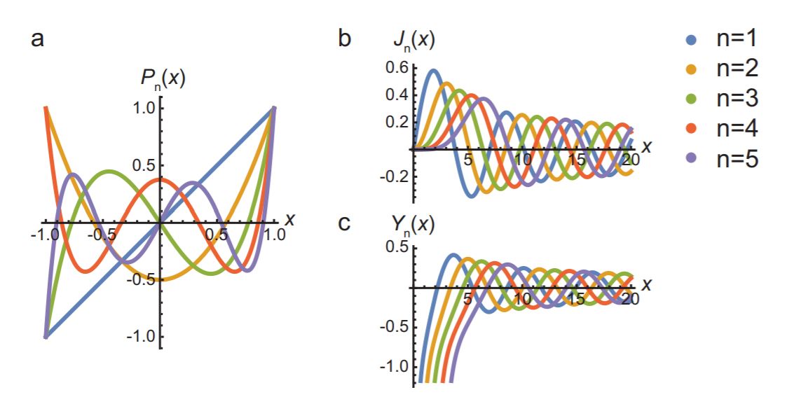
Given the values of \(a_0\) and \(a_1\) (the two degrees of freedom that our second-order differential equation allows us), we can repeatedly apply Equation \ref{A.43} to get all coefficients. Note that for \(k = n\) the coefficient equals zero. Therefore, if for an even value of \(n\), we set \(a_1 = 0\), and for an odd value of \(n\), we set \(a_0 = 0\), we get a finite number of nonzero coefficients. The resulting solutions are polynomials, characterized by the number \(n\); in this case, they’re known as the Legendre polynomials, typically denoted \(P_n (x)\), and normalized (by setting the value of the remaining free coefficient) such that \(P_n (1) = 1\). Table A.1 lists the first five, which are also plotted in Figure 16.A.4a.
Legendre polynomials have many other interesting properties (many of which can be found in either math textbooks or on their Wikipedia page). They occur frequently in physics, for example in solving problems involving Newtonian gravity or Laplace’s equation from electrostatics.
If we replace the \(n(n + 1)\) factor in the Legendre differential equation with an arbitrary number \(\lambda\), the series solution remains a solution, but it no longer terminates8. There are many other differential equations that lead to both infinite series and polynomial solutions. A well-known example is the Bessel differential equation:
\[x^{2} \frac{\mathrm{d}^{2} y}{\mathrm{d} x^{2}}+x \frac{\mathrm{d} y}{\mathrm{d} x}+\left(x^{2}-n^{2}\right) y(x)=0 \label{A.44}\]
The solutions to this equation are known as the Bessel functions of the first and second kind (see Problem A.3.3, where you’ll prove that for these functions the series never terminates). These functions generalize the sine and cosine function and occur in the vibrations of two-dimensional surfaces. Other examples include the Hermite and Laguerre polynomials, which feature in quantum mechanics, and Airy functions, which you can encounter when studying optics.
| \(n\) | \(P_n (x)\) |
|---|---|
| 0 | 1 |
| 1 | x |
| 2 | \(\frac{1}{2}(3 x-1)\) |
| 3 | \(\frac{1}{2}\left(5 x^{3}-3 x\right)\) |
| 4 | \(\frac{1}{8}\left(35 x^{4}-30 x^{2}+3\right)\) |
| 5 | \(\frac{1}{8}\left(63 x^{5}-70 x^{3}+15 x\right)\) |
A.3.6. Problems
A.3.1
- Suppose we have a solution of Equation \ref{A.24} where the roots \(\lambda _{\pm}\) of the characteristic polynomial (Equation \ref{A.26}) are complex, so \(\lambda _{\pm} = \alpha \pm i \beta\). Rewrite the general solution \ref{A.27} in real functions with real coefficients C and D, and express C and D in terms of A and B. Hint: use Euler’s formula \(e^{i x}=\cos (x)+i \sin (x)\).
- Suppose we have a solution of Equation \ref{A.32} where the roots \(n _{\pm}\) are complex, so \(n_{\pm} = \alpha \pm i \beta\). To get a solution of Equation \ref{A.30} without complex numbers, we make the substitution \(x = e^t\), so \[x^{n_{\pm}}=x^{\alpha \pm i \beta}=e^{\alpha t} e^{\pm i \beta t}\] Use Euler’s formula again to rewrite the complex exponential in terms of sines and cosines, and make the back-substitution to x to show that the general solution of Equation \ref{A.30} in this case is given by \[y(x)=x^{\alpha}[A \cos (\beta \ln (x))+\sin (\beta \ln (x))]\]
- Suppose we have a solution of Equation \ref{A.32} for which there is only a single root n. Show that the derivative of \(x^n\) with respect to n is in this case also a solution of Equation \ref{A.30}, and that the general solution is given by \[y(x)=x^{n}[A+B \ln (x)]\]
A.3.2 Use the method of reduction of order to obtain a second solution of Equation \ref{A.24} for the case that the characteristic polynomial (Equation \ref{A.26}) has only a single root.
A.3.3
- Use the power series technique to find a solution to Bessel’s differential Equation \ref{A.44}. Why doesn’t the series terminate in this case? Why do you only get one family of solutions? We’ll call these solutions ‘Bessel functions of the first kind’ and label them as \(J_n (x)\) (see Figure 16.A.4b).
- Use the method of reduction of order to find a second family of solutions to the Bessel differential equation, known as ‘Bessel functions of the second kind’ (\(Y_n (x)\), see Figure 16.A.4c).