15.3: Charged Particle Motion

We now explore some examples of the motion of charged particles under the influence of electric and magnetic fields.

Particle in Constant Electric Field

Suppose a particle with charge q is exposed to a constant electric field \(\mathrm{E}_{\mathrm{x}}\) in the \(x\) direction. The \(x\) component of the force on the particle is thus \(\mathrm{F}_{\mathrm{x}}=\mathrm{q} \mathrm{E}_{\mathrm{x}}\). From Newton’s second law the acceleration in the \(x\) direction is therefore \(a_{x}=F_{x} / m=q E_{x} / m\) where \(m\) is the mass of the particle. The behavior of the particle is the same as if it were exposed to a constant gravitational field equal to \(\mathrm{qE}_{\mathrm{x}} / \mathrm{m}\).

Particle in Conservative Electric Field

If \(\partial \mathbf{A} / \partial \mathrm{t}=0\), then the electric force on a charged particle is

\[\mathbf{F}_{\text {electric }}=-q\left(\frac{\partial \phi}{\partial x}, \frac{\partial \phi}{\partial y}, \frac{\partial \phi}{\partial z}\right), \quad \frac{\partial \mathbf{A}}{\partial t}=0\label{15.7}\]

This force is conservative, with potential energy \(\mathrm{U}=\mathrm{q} \phi .\). Recalling that the total energy, \(\mathrm{E}=\mathrm{K}+\mathrm{U},\), of a particle under the influence of a conservative force remains constant with time, we can infer that the change in the kinetic energy with position of the particle is just minus the change in the potential energy: \(\Delta \mathrm{K}=-\Delta \mathrm{U}\). Notice in particular that if the particle returns to its initial position, the change in the potential energy is zero and the kinetic energy recovers its initial value.

If \(\partial \mathbf{A} / \partial \mathrm{t} \neq 0\), then there is the possibility that the electric force is not conservative. Recall that the magnetic field is derived from A. Interestingly, a necessary and sufficient criterion for a non-conservative electric force is that the magnetic field be changing with time. This result was first inferred experimentally by the English physicist Michael Faraday in 1831 and at nearly the same time by the American physicist Joseph Henry. It will be further explored later in this chapter.

Torque on an Electric Dipole

Let us now imagine a “dumbbell” consisting of positive and negative charges of equal magnitude q separated by a distance d, as shown in figure 15.1. If there is a uniform electric field E, the positive charge experiences a force \(\text { qE }\), while the negative charge experiences a force \(\text {-qE }\). The net force on the dumbbell is thus zero.

Figure 15.1: Definition sketch for an electric dipole. Two charges, q and -q are connected by an uncharged bar of length \(d\). The vectors \(\text { d / } 2\) and \(\text {-d / } 2\) give the positions of the two charges relative to the central point between them. The two forces are due to the electric field E.

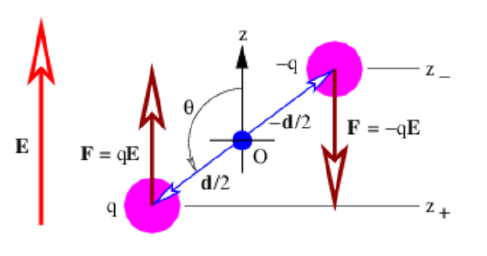
The torque acting on the dumbbell is not zero. The total torque acting about the origin in figure 15.1 is the sum of the torques acting on the two charges:

\[\boldsymbol{\tau}=(-q)(-\mathbf{d} / 2) \times \mathbf{E}+(q)(\mathbf{d} / 2) \times(\mathbf{E})=q \mathbf{d} \times \mathbf{E}\label{15.8}\]

The vector d can be thought of as having a length equal to the distance between the two charges and a direction going from the negative to the positive charge.

The quantity \(\mathbf{p}=q \mathbf{d}\) is called the electric dipole moment. (Don’t confuse it with the momentum!) The torque is just

\[\boldsymbol{\tau}=\mathbf{p} \times \mathbf{E}\label{15.9}\]

This shows that the torque depends on the dipole moment, or the product of the charge and the separation. Thus, halving the separation and doubling the charge results in the same dipole moment.

The tendency of the torque is to rotate the dipole so that the dipole moment p is parallel to the electric field E. The magnitude of the torque is given by

\[\tau=p E \sin (\theta)\label{15.10}\]

where the angle θ is defined in figure 15.1 and \(p=|\mathbf{p}|\) is the magnitude of the electric dipole moment.

The potential energy of the dipole is computed as follows: The scalar potential associated with the electric field is \(\phi=-E z\) where E is the magnitude of the field, assumed to point in the +z direction. Thus, the potential energy of a single particle with charge q is \(U=q \phi=-\mathrm{q} \mathrm{Ez}\). The total potential energy of the dipole is the sum of the potential energies of the individual charges:

\[\begin{aligned}
U &=(+q)\left(-E z_{+}\right)+(-q)\left(-E z_{-}\right)=-q E\left(z_{+}-z_{-}\right) \\
&=-q E d \cos (\theta)=-p E \cos (\theta)=-\mathbf{p} \cdot \mathbf{E}
\end{aligned}\label{15.11}\]

where z₊ and z_- are the z positions of the positive and negative charges. The equating of z₊ - z_- to \(\mathrm{d} \cos (\theta)\) may be verified by examining the geometry of figure 15.1.

The tendency of the electric field to align the dipole moment with itself is confirmed by the potential energy formula. The potential energy is lowest when the dipole moment is aligned with the field and highest when the two are anti-aligned.

Particle in Constant Magnetic Field

The magnetic force on a particle with charge \(q\) moving with velocity v is \(\mathbf{F}_{\text {magnetic }}=\mathrm{q} \mathbf{v} \times \mathbf{B}\), where \(B\) is the magnetic field. The magnetic force is directed perpendicular to both the magnetic field and the particle’s velocity. Because of the latter point, no work is done on the particle by the magnetic field. Thus, by itself the magnetic force cannot change the magnitude of the particle’s velocity, though it can change its direction.

Figure 15.2: Spiraling motion of a charged particle in the direction of the magnetic field. This is composed of a circular motion about the field vector plus a translation along the field.

If the magnetic field is constant, the magnitude of the magnetic force on the particle is also constant and has the value \(F_{\text {magnetic }}=\operatorname{gvB} \sin (\theta)\) where \(v=|\mathbf{v}|, \mathrm{B}=|\mathbf{B}|\), and \(\theta\) is the angle between v and B. If the initial velocity is perpendicular to the magnetic field, then \(\sin (\theta)=1\) and the force is just \(\mathrm{F}_{\text {magnetic }}=\mathrm{qvB}\). The particle simply moves in a circle with the magnetic force directed toward the center of the circle. This force divided by the mass m must equal the particle’s centripetal acceleration: \(\mathrm{v}^{2} / \mathrm{R}=\mathrm{a}=\mathrm{F}_{\text {magnetic }} / \mathrm{m}=\mathrm{qvB} / \mathrm{m}\) in the non-relativistic case, where \(R\) is the radius of the circle. Solving for \(R\) yields

\[R=m v /(q B)\label{15.12}\]

The angular frequency of revolution is

\[\omega=v / R=q B / m \quad \text { (cyclotron frequency). }\label{15.13}\]

Notice that this frequency is a constant independent of the radius of the particle’s orbit or its velocity. This is called the cyclotron frequency.

If the initial velocity is not perpendicular to the magnetic field, then the particle still has a circular component of motion in the plane normal to the field, but also drifts at constant speed in the direction of the field. The net result is a spiral motion in the direction of the magnetic field, as illustrated in figure 15.2. The radius of the circle is \(\mathrm{R}=\mathrm{mv}_{\mathrm{p}} /(\mathrm{qB})\) in this case, where \(\mathrm{v}_{\mathrm{p}}\) is the component of \(v\) perpendicular to the magnetic field.

Crossed Electric and Magnetic Fields

If we have perpendicular electric and magnetic fields as shown in figure 15.3, then it is possible for a charged particle to move such that the electric and magnetic forces simply cancel each other out. From the Lorentz force equation (15.2.3), the condition for this happening is \(\mathbf{E}+\mathbf{v} \times \mathbf{B}=0\). If \(E\) and \(B\) are perpendicular, then this equation requires v to point in the direction of \(\mathbf{E} \times \mathbf{B}\) (i. e., normal to both vectors) with the magnitude \(\mathrm{V}=|\mathbf{E}| /|\mathbf{B}|\). This, of course, is not the only possible motion under these circumstances, just the simplest.

Figure 15.3: With crossed electric \(E\) and magnetic \(B\) fields (i. e., fields perpendicular to each other), a charged particle can move at a constant velocity v with magnitude equal to \(v=|E| /|B|\) and direction perpendicular to both \(E\) and \(B\). This is because the electric and magnetic forces, \(F_{\text {electric }}=q \mathrm{E} \text { and } F_{\text {magnetic }}=q v \times B\), balance each other in this case.

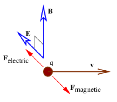
It is interesting to consider this situation from the point of view of a reference frame that is moving with the charged particle. In this reference frame the particle is stationary and therefore not subject to the magnetic force. Since the particle is not accelerating, the net force, which in this frame consists only of the electric force, is zero. Hence, the electric field must be zero in the moving reference frame.

Figure 15.4: The four-potential a and its components in two different reference frames. In the unprimed frame the four-potential is purely space-like. The primed frame is moving in the \(x\) direction at speed \(U\) relative to the unprimed frame. The four-potential points along the \(x\) axis.

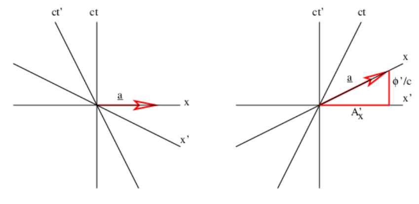
This argument shows that the electric field perceived in one reference frame is not necessarily the same as the electric field perceived in another frame. Figure 15.4 shows why this is so. The left panel shows the situation in the reference frame moving to the right, which is the unprimed frame in this picture. The charged particle is stationary in this reference frame. The four-potential is purely spacelike, having no time component \(\phi / \mathrm{c} .\). Assuming that a is constant in time, there is no electric field, and hence no electric force. Since the particle is stationary in this frame, there is also no magnetic force. However, in the primed reference frame, which is moving to the left relative to the unprimed frame and therefore is equivalent to the original reference frame in which the particle is moving to the right, the four-potential has a time component, which means that a scalar potential and hence an electric field is present.