16.2: Gauss’s Law for Electricity

Last updated
Save as PDF

Page ID: 32843

\( \newcommand{\vecs}[1]{\overset { \scriptstyle \rightharpoonup} {\mathbf{#1}} } \) \( \newcommand{\vecd}[1]{\overset{-\!-\!\rightharpoonup}{\vphantom{a}\smash {#1}}} \)\(\newcommand{\id}{\mathrm{id}}\) \( \newcommand{\Span}{\mathrm{span}}\) \( \newcommand{\kernel}{\mathrm{null}\,}\) \( \newcommand{\range}{\mathrm{range}\,}\) \( \newcommand{\RealPart}{\mathrm{Re}}\) \( \newcommand{\ImaginaryPart}{\mathrm{Im}}\) \( \newcommand{\Argument}{\mathrm{Arg}}\) \( \newcommand{\norm}[1]{\| #1 \|}\) \( \newcommand{\inner}[2]{\langle #1, #2 \rangle}\) \( \newcommand{\Span}{\mathrm{span}}\) \(\newcommand{\id}{\mathrm{id}}\) \( \newcommand{\Span}{\mathrm{span}}\) \( \newcommand{\kernel}{\mathrm{null}\,}\) \( \newcommand{\range}{\mathrm{range}\,}\) \( \newcommand{\RealPart}{\mathrm{Re}}\) \( \newcommand{\ImaginaryPart}{\mathrm{Im}}\) \( \newcommand{\Argument}{\mathrm{Arg}}\) \( \newcommand{\norm}[1]{\| #1 \|}\) \( \newcommand{\inner}[2]{\langle #1, #2 \rangle}\) \( \newcommand{\Span}{\mathrm{span}}\)\(\newcommand{\AA}{\unicode[.8,0]{x212B}}\)

The electric flux is defined in analogy to the gravitational flux as

\[ \Phi_{E}=\mathbf{S} \cdot \mathbf{E} \quad(\text { electric flux }) \label{16.5}\]

where \(S\) is the directed area through which the flux passes. (This is strictly true only for small, flat areas \(S\) over which the component of \(E\) normal to \(S\) can be assumed constant.) Since the electric field obeys an inverse square law, Gauss’s law applies to the electric flux Φ_E just as it applies to the gravitational flux. In particular, since the magnitude of the outward electric field a distance \(r\) from a charge \(q \text { is } E=q\left(4 \pi \epsilon_{0} r^{2}\right)\), the electric flux through a sphere of radius \(r\) (and area \(4 \pi r^{2}\)) concentric with the charge is \(E S=\left[q\left(4 \pi \epsilon_{0} r^{2}\right)\right] \times\left(4 \pi r^{2}\right)=q / \epsilon_{0}\). This generalizes to an arbitrary distribution of charge as in the gravitational case:

\[\Phi_{E}=q_{\text {inside }} / \epsilon_{0} \quad \text { (Gauss's law for electricity), }\label{16.6}\]

where Φ_E in this equation is the outward electric flux through a closed surface and \(q_{\text {inside }}\) is the net charge inside this surface. This is an expression of Gauss’s law for the electric field. Since Gauss’s law for electricity and for gravitation are so similar, we can use all our insights from studying gravity on the electric field case.

Sheet of Charge

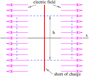
Figure 16.1: Definition sketch for use of Gauss’s law to obtain the electric field due to an infinite sheet of surface charge. The dashed line shows the Gaussian box, which is of height \(h \) and depth \(d \) into the page.

Figure 16.1 shows how to set up the Gaussian surface to obtain the electric field emanating from an infinite sheet of charge. We assume a charge density of \(σ \) Coulombs per square meter, which means that the amount of charge inside the box is \(q\) _inside = \(σhd\), where the box has height \(h \) and depth \(d\) into the page. The total electric flux out of the left and right faces of the box is Φ_E = 2\(Ehd\), where \(E \) is the magnitude of the electric field on these surfaces. The field is assumed to point away from the charge, and hence out of the box on both faces. Due to the assumed direction of the electric field, there is no electric flux out of any of the other faces of the box.

Applying Gauss’s law, we infer that \(2 E h d=\sigma h d \epsilon_{0}\), which means that the electric field emanating from a sheet of charge with charge density per unit area \(σ\) is

\[E=\frac{\sigma}{2 \epsilon_{0}}\label{16.7}\]

The scalar potential associated with this electric field is easily obtained by realizing that Equation \ref{16.7} gives the \(x \) component of this field — the other components are zero. Using \(E=-\partial \phi / \partial x\), we infer that

\[ \phi=-\frac{\sigma|x|}{2 \epsilon_{0}}\label{16.8}\]

The absolute value signs around \(x\) take account of the fact that the direction of the electric field for negative \(x\) is opposite that for positive \(x\).

Line of Charge

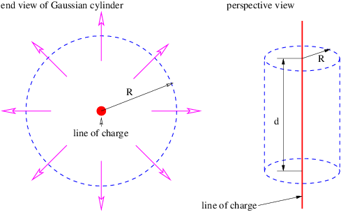
Figure 16.2: Definition sketch for use of Gauss’s law to obtain the electric field due to an infinite line charge oriented normal to the page. The dashed line shows the Gaussian cylinder, which is of radius \(R\) and length \(d\) into the page. The outward-pointing arrows show the electric field.

Similar reasoning is used to obtain the electric field due to a line of charge. A sketch of the expected electric field vectors and a Gaussian cylinder coaxial with the line of charge is shown in figure 16.2. If the charge per unit length is \(λ\), the amount of charge inside the cylinder is \(q_{\text {inside }}=\lambda d\), where \(d\) is the length of the cylinder. The outward electric flux at radius \(r\) is \(\Phi_{E}=2 \pi r d E\). Gauss’s law therefore tells us that the electric field at radius \(r\) is just

\[E=\frac{\lambda}{2 \pi \epsilon_{0} r}\label{16.9}\]

In this case \(E=-\partial \phi / \partial r,\), so that the scalar potential is

\[\phi=-\frac{\lambda}{2 \pi \epsilon_{0}} \ln (r).\label{16.10}\]