24.1: Ideal Gas

An ideal gas is an assembly of atoms or molecules that interact with each other only via occasional collisions. The distance between molecules is much greater than the range of inter-molecular forces, so gas molecules behave as free particles most of the time. We assume here that the density of molecules is also low enough to make the probability of finding more than one molecule in a given quantum mechanical state very small. For this reason it doesn’t matter whether the molecules are bosons or fermions for our calculations.

J. Willard Gibbs tried computing the entropy of an ideal gas using his version of statistical mechanics, which was based on classical mechanics. The result was wrong in a very fundamental way — the calculated amount of entropy was not proportional to the amount of gas. In fact, the amount of entropy of an ideal gas at fixed temperature and pressure is calculated to have a non-linear dependence on the number of gas molecules. In particular, doubling the amount of gas more than doubles the entropy according to the Gibbs formula.

Figure 24.1: Consequence of the incorrect classical calculation of entropy of an ideal gas by Gibbs. Two parts of a container separated by a divider each contain the same type of gas at the same temperature and pressure. The total entropy is 2S where S is the classically calculated entropy of each half. If the divider is removed, the classical calculation yields an entropy for the entire body of gas S′ > 2S. Reinserting the divider returns the container to the initial state in which the total entropy is 2S.

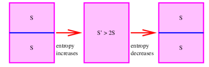
The significance of this error is illustrated in figure 24.1. Imagine a container of gas of a certain type, temperature, and pressure that is divided into two equal parts by a sheet of material. The total entropy of this state is 2S, where S is the entropy calculated separately for each half of the body of gas. This follows because the two halves are completely separate systems.

If the divider is now removed, a calculation of the entropy of the full body of gas yields S′ > 2S according to the Gibbs formula, since the calculated entropy doesn’t scale with the amount of gas. Furthermore, replacing the divider restores the system to the initial state in which the total entropy is 2S. Thus, simply inserting or removing the divider, an operation that transfers no heat and does no work on the system, is able to increase or decrease the entropy of the gas at will according to Gibbs. This is at variance with the second law of thermodynamics and is known not to occur. Its prediction by the formula of Gibbs is called the Gibbs paradox. Gibbs was well aware of the serious nature of this problem but was unable to come up with a satisfying solution.

The resolution of the paradox is simply that the Gibbs formula for the entropy of an ideal gas is incorrect. The correct formula is only obtained when the quantum mechanical version of statistical mechanics is used. The failure of Gibbs to obtain the proper entropy was an early indication that classical mechanics had problems on the atomic scale.

We will now calculate the entropy of a body of ideal gas using quantum statistical mechanics. In order to reduce the difficulty of the calculation, we will take a shortcut and assume that the amount of entropy is proportional to the amount of gas. However, the more rigorous calculation confirms that this actually is true.

Particle in a Three-Dimensional Box

The quantum mechanical calculation of the states of a particle in a three-dimensional box forms the basis for our treatment of an ideal gas. Recall that a non-relativistic particle of mass M in a one-dimensional box of width a can only support wavenumbers \(k_{l}=\pm \pi l/a\) where l = 1, 2, 3,… is the quantum number for the particle. Thus, the possible momenta are \(p_{l}=\pm \hbar \pi l / a\) and the possible energies are

\[E_{l}=p_{l}^{2} /(2 M)=\hbar^{2} \pi^{2} l^{2} /\left(2 M a^{2}\right) \quad \text { (one-dimensional box) }\label{24.1}\]

If the box has three dimensions, is cubical with edges of length a, and has one corner at (x,y,z) = (0, 0, 0), the quantum mechanical wave function for a single particle that satisfies ψ = 0 on all the walls of the box is a three-dimensional standing wave,

\[\psi(x, y, z)=\sin (l x \pi / a) \sin (m y \pi / a) \sin (n z \pi / a)\label{24.2}\]

where the quantum numbers l,m,n are positive integers. You can verify this by examining ψ for x = 0, x = a, etc.

Equation (\ref{24.2}) is a solution in which the x, y, and z wavenumbers are respectively \(k_{x}=\pm l \pi d a, k_{y}=\pm m \pi a, \text { and } k_{z}=\pm n \pi / a\). The corresponding components of the kinetic momentum are therefore \(p_{x}=\hbar k_{x}\) etc. The possible energy values of the particle are

\[\begin{equation}
\begin{aligned}
E_{l m n} &=\frac{p^{2}}{2 M}=\frac{p_{x}^{2}+p_{y}^{2}+p_{z}^{2}}{2 M}=\frac{\hbar^{2} \pi^{2}\left(l^{2}+m^{2}+n^{2}\right)}{2 M a^{2}} \\
&=\frac{\hbar^{2} \pi^{2} L^{2}}{2 M V^{2/3}} \equiv E_{0} L^{2} \quad(\text { three-dimensional box }) .
\end{aligned}
\end{equation}\label{24.3}\]

In the last line of the above equation we have eliminated the linear dimension a of the box in favor of its volume V = a³ and have adopted the shorthand notation \(\mathrm{L}^{2}=\mathrm{l}^{2}+\mathrm{m}^{2}+\mathrm{n}^{2}\) and \(E_{0}=\hbar^{2} \pi^{2} /\left(2 M a^{2}\right)=\hbar^{2} \pi^{2} /\left(2 M V^{2 \3}\right)\). The quantity \(E_{0}\) is the ground state energy for a particle in a one-dimensional box of size \(a\).

Figure 24.2: Energy levels for a non-relativistic particle in a one-dimensional and a three-dimensional box, each of side length a. The value E₀ is the ground state energy of the one-dimensional particle in a box of length a. The numbers to the right of the levels respectively give the values of l for the 1-D oscillator and the values of l, m, and n for the 3-D oscillator. The numbers in parentheses give the degeneracy of each energy level (see text).

Figure 24.2 shows the energy levels of a particle in a one-dimensional and a three-dimensional box. Different values of l, m, and n can result in the same energy in the three-dimensional case. For instance, (l,m,n) = (1, 1, 2), (1, 2, 1), (2, 1, 1) all yield L² = 6 and hence energy 6\(E_{0}\). This energy level is thus said to have a degeneracy of 3. Similarly, the states (1, 2, 3), (2, 3, 1), (3, 1, 2), (3, 2, 1), (2, 1, 3), (1, 3, 2) all have the same value of L², so this level has a degeneracy of 6. However, the state (1, 1, 1) is unique and thus has a degeneracy of 1. From this we see that the degeneracy of an energy level is the number of different physically distinguishable states that have the same energy. Counting the effects of degeneracy, the particle in a three-dimensional box has 60 distinct states for energy less than 30\(E_{0}\), while the one-dimensional box has 5. As \(E/E_{0}\) increases, this ratio becomes even larger.

Counting States

Figure 24.3: The states of a particle in a two-dimensional box. The dots indicate particular states associated with allowed values of the x and y direction quantum numbers, l and m. The pie-shaped segment bounded by the arc of radius L and the l and m axes encompasses all of the states with \(\mathrm{I}^{2}+\mathrm{m}^{2} \leq \mathrm{L}^{2}\).

In order to compute the entropy of a system, we need to count the number of states available to the system in a particular band of energies. Figure 24.3 shows how to count the states with energy less than some limiting value for a particle in a two-dimensional box. The pie-shaped segment bounded by the arc of radius L and the l and m axes has an area equal to one fourth the area of a circle of radius \(L\), or \(\pi L^{2} / 4\). The dots represent allowed values of the l and m quantum numbers. One dot, and hence one state, exists per unit area in this graph, so the above expression tells us how many states \(\mathcal{N}\) exist with \(l^{2}+m^{2} \leq L^{2}\)

In two dimensions the particle energy is \(E=\left(l^{2}+m^{2}\right) E_{0}\). Thus, the number of states with energy less than or equal to some maximum energy \(E\) is

\[\mathcal{N}=\frac{\pi L^{2}}{4}=\frac{\pi}{4}\left(\frac{E}{E_{0}}\right) \quad \text { (two-dimensional box). }\label{24.4}\]

Similar arguments can be made to calculate the number of states of a particle in a three-dimensional box. The equivalent of figure 24.3 would be a plot with three axes, l, m, and n representing the \(x\), \(y\), and \(z\) quantum numbers. The volume of a sphere with radius L is then \(4 \Pi L^{3} / 3\) and the region of the sphere with l,m,n > 0, i. e., an eighth of the sphere, contains real physical states. The result is that

\[\mathcal{N}=\frac{4 \pi L^{3}}{3 \cdot 8}=\frac{\pi}{6}\left(\frac{E}{E_{0}}\right)^{3 / 2} \quad(\text { three-dimensional box })\label{24.5}\]

states exist with energy less than E.

Multiple Particles

An ideal gas of only one molecule isn’t very interesting. Calculating the number of states available to many particles in a box is a bit complex. However, by analogy with the case of multiple harmonic oscillators, we guess that the number of states of an N-particle gas is the number of states available to a single particle to the Nth power multiplied by some as yet unknown function of N, F(N):

\[\mathcal{N}=F(N)\left(\frac{E}{E_{0}}\right)^{3 N / 2} \quad(N \text { particles in 3-D box })\label{24.6}\]

(Note that the \((п / 6)^{N}\) from equation (\ref{24.5}) has been absorbed into F(N).) Substituting \(\mathrm{E}_{0}=\hbar^{2} \Pi^{2} /\left(2 \mathrm{MV}^{2 / 3}\right)\) results in

\[\mathcal{N}=F(N)\left(\frac{2 M E V^{2 / 3}}{\hbar^{2} \pi^{2}}\right)^{3 N / 2}\label{24.7}\]

Now, \(\Pi^{2} \hbar^{2} /(2 M)\) has the units of energy multiplied by volume to the two-thirds power, so we write this combination of constants in terms of constant reference values of E and V :

\[\pi^{2} \hbar^{2} /(2 M)=E_{r e f} V_{r e f}^{2 / 3}\label{24.8}\]

Given the above assumption, we can rewrite the number of states with energy less than E as

\[\mathcal{N}=F(N)\left(\frac{E}{E_{r e f}}\right)^{3 N / 2}\left(\frac{V}{V_{r e f}}\right)^{N}\label{24.9}\]

We now argue that the combination F(N) must take the form KN^-5N∕2 where K is a dimensionless constant independent of N. Substituting this assumption into equation (\ref{24.9}) results in

\[\mathcal{N}=K\left(\frac{E}{N E_{r e f}}\right)^{3 N / 2}\left(\frac{V}{N V_{r e f}}\right)^{N} .\label{24.10}\]

It turns out that we will not need the actual values of any of the three constants \(K\), \(\mathrm{E}_{\mathrm{ref}}\), or \(V_{\text {ref }}\).

The effect of the above hypothesis is that the energy and volume occur only in the combinations \(\mathrm{E} /\left(\mathrm{NE}_{\mathrm{ref}}\right)\) and \(\mathrm{V} /\left(\mathrm{NV}_{\text {ref }}\right) \text { . }\). First of all, these combinations are dimensionless, which is important because they will become the arguments of logarithms. Second, because of the N in the denominator in both cases, they are in the form of energy per particle and volume per particle. If the energy per particle and the volume per particle stay fixed, then the only dependence of \(\mathcal{N}\) on N is via the exponents 3N∕2 and N in the above equation. Why is this important? Read on!

Entropy and Temperature

Recall now that we need to compute the number of states in some small energy interval ΔE in order to get the entropy. Proceeding as for the case of a collection of harmonic oscillators, we find that

\[\Delta \mathcal{N}=\frac{\partial \mathcal{N}}{\partial E} \Delta E=\frac{3 K N \Delta E}{2 E}\left(\frac{E}{N E_{r e f}}\right)^{3 N / 2}\left(\frac{V}{N V_{r e f}}\right)^{N}\label{24.11}\]

The entropy is therefore

\[S=k_{B} \ln (\Delta \mathcal{N})=N k_{B}\left[\frac{3}{2} \ln \left(\frac{E}{N E_{r e f}}\right)+\ln \left(\frac{V}{N V_{r e f}}\right)\right] \quad \text { (ideal }\label{24.12}\]

where we have dropped the term \(\mathrm{k}_{\mathrm{B}} \ln [3 \mathrm{KN} \Delta \mathrm{E} /(2 \mathrm{E})]\). Since this term is not multiplied by the number of particles N, it is unimportant for systems made up of lots of particles.

Notice that this equation has a very important property, namely, that the entropy is proportional to the number of particles for fixed \(\mathrm{E} / \mathrm{N} \text { and } \mathrm{V} / \mathrm{N}\). It thus satisfies the criterion that Gibbs was unable to satisfy in his computation of the entropy of an ideal gas. However, we cannot claim that our calculation is superior to his, because we cheated! The reason we assumed that \(\mathrm{F}(\mathrm{N})=\mathrm{KN}^{-5 \mathrm{~N} / 2}\) is precisely so that we would obtain this result.

The temperature is the inverse of the E-derivative of entropy:

\[\frac{1}{T}=\frac{\partial S}{\partial E}=\frac{3 N k_{B}}{2 E} \quad \Longrightarrow \quad T=\frac{2 E}{3 N k_{B}} \quad \text { or } \quad E=\frac{3 N k_{B} T}{2} .\label{24.13}\]

Slow and Fast Expansions

How does the entropy of a particle in a box change if the volume of the box is changed? The answer to this question depends on how rapidly the volume change takes place. If an expansion or compression takes place slowly enough and no heat is added or removed, the quantum numbers of the particle don’t change.

Figure 24.4: Harmonics on a guitar. Plucking a string while a finger rests lightly on the string at the 12th fret results in excitation of the first harmonic on the guitar string. Only one string is shown for clarity.

____________________________

---

This fact may be demonstrated by the tuning of a guitar. A guitar string is tuned in frequency by adjusting the tension on the string with the tuning peg. If the first harmonic mode (corresponding to quantum number n = 2 for particle in a one-dimensional box) is excited on a guitar string as illustrated in figure 24.4, changing the tension changes the frequency of the vibration but it does not change the mode of vibration of the string — for instance, if the first harmonic is initially excited, it remains the primary mode of oscillation.

Slowly changing the volume of a gas consisting of many particles, each with its own set of quantum numbers, results in the same behavior — changing the dimensions of the box results in no switching of quantum numbers beyond that which would normally take place as a result of particle collisions. As a consequence, the number of states available to the system, \(\Delta \mathcal{N},\), and hence the entropy, doesn’t change either.

A process that changes the macroscopic condition of a system but that doesn’t change the entropy is called isentropic or reversible adiabatic. The word “isentropic” means at constant entropy, while “adiabatic” means that no heat flows in or out of the system.

Figure 24.5: The curved line indicates the reversible adiabatic curve E ∝ V ^-2∕3 for an ideal gas in a box. The two straight line segments indicate what happens in a rapid expansion or compression.

____________________________

---

If the entropy doesn’t change as a result of a change in volume, then E^3∕2V = const according to equation (\ref{24.12}). Thus, the energy of the gas increases when the volume is decreased and vice versa. This behavior is illustrated in figure 24.5. The change in energy in both cases is a consequence of work done by the gas on the walls of the container as it changes volume — positive in expansion, meaning that the gas loses energy; and negative in compression, meaning that the gas gains energy. This type of energy transfer is the means by which internal energy is converted to useful work.

A rapid expansion of the box has a completely different effect. If the expansion is so rapid that the quantum mechanical waves trapped in the box undergo negligible evolution during the expansion, then the internal energy of the particles in the box does not change. As a consequence, the particle quantum numbers must change to compensate for the change in volume. Equation (\ref{24.12}) tells us that if the volume increases and the internal energy doesn’t change, the entropy must increase.

A rapid compression has the opposite effect — it does extra work on the material in the box, thus adding internal energy to the gas at a rate in excess of the reversible adiabatic rate. The entropy increases in this type of process as well. Both of these effects are illustrated in figure 24.5.

Work, Pressure, and Gas Law

The pressure p of a gas is the normal force per unit area exerted by the gas on the walls of the chamber containing the gas. If a chamber wall is movable, the pressure force can do positive or negative work on the wall if it moves out or in. This is the mechanism by which internal energy is converted to useful work. We can determine the pressure of a gas from the entropy formula.

Figure 24.6: Gas in a cylinder with a movable piston. The force F exerted by the gas on the piston is the area A of the face of the piston multiplied by the pressure p.

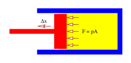
Consider the behavior of a gas contained in a cylinder with a movable piston as shown in figure 24.6. The net force F exerted by gas molecules bouncing off of the piston results in work ΔW = FΔx being done by the gas if the piston moves (slowly) out a distance Δx. The pressure is related to F and the area A of the piston by \(p=F / A\). Furthermore, the change in volume of the cylinder is \(\Delta \mathrm{V}=\mathrm{A} \Delta \mathrm{x}\).

If the gas does work \(\Delta \mathrm{W}\) on the piston, its internal energy changes by

\[\Delta E=-\Delta W=-F \Delta x=-\frac{F}{A} A \Delta x=-p \Delta V\label{24.14}\]

assuming that ΔQ = 0, i. e., no heat is added or removed during the change in volume. Solving this for p results in

\[p \equiv-\frac{\partial E}{\partial V}\label{24.15}\]

In the previous section we showed that as long as the change in volume is slow and ΔQ = 0, the entropy does not change. Thus, in the evaluation of \(\partial \mathrm{E} / \partial \mathrm{V} \text { , }\), the entropy is held constant.

We can determine the pressure for an ideal gas by solving equation (\ref{24.12}) for \(E\) and taking the \(V\) derivative. As we showed in the previous section, \(\mathrm{E}^{3 / 2} \mathrm{~V}\) is constant for constant entropy processes, which means that

\[E=B V^{-2 / 3} \quad \text { (constant entropy expansion) }\label{24.16}\]

where B is constant.

The pressure is then computed to be

\[p=-\frac{\partial E}{\partial V}=\frac{2}{3} \frac{B}{V^{5 / 3}}=\frac{2 E}{3 V} \quad \text { (ideal gas), }\label{24.17}\]

where B is eliminated in the last step using equation (\ref{24.16}). Employing equation (\ref{24.13}) to eliminate the energy in favor of the temperature, this can be written

\[p V=N k_{B} T \quad \text { (ideal gas law) }\label{24.18}\]

which relates the pressure, volume, temperature, and particle number of an ideal gas.

This equation is called the ideal gas law and jointly represents the observed relationships between pressure and volume at constant temperature (Boyle’s law) and pressure and temperature at constant volume (law of Charles and Gay-Lussac). The fact that we can derive it from statistical mechanics is evidence in favor of our quantum mechanical model of a gas.

The formulas for the entropy of an ideal gas (\ref{24.12}), its temperature (\ref{24.13}), and the ideal gas law (\ref{24.18}) summarize our knowledge about ideal gases. Actually, the entropy and temperature laws only apply to a particular type of ideal gas in which the molecules consist of single atoms. This is called a monatomic ideal gas, examples of which are helium, argon, and neon. The molecules of most gases consist of two or more atoms. These molecules have rotational degrees of freedom that can store energy. The calculation of the entropy of such gases needs to take these factors into account. The most common case is one in which the molecules are diatomic, i. e., they consist of two atoms each. In this case simply replacing factors of \(3 / 2 \text { by } 5 / 2\) in equations (\ref{24.12}), (\ref{24.13}), (\ref{24.16}), and (\ref{24.17}) results in equations that apply to diatomic gases at ordinary temperatures.

Specific Heat of an Ideal Gas

As previously noted, the specific heat of any substance is the amount of heating required per unit mass to raise the temperature of the substance by one degree. For a gas one must clarify whether the volume or the pressure is held constant as the temperature increases — the specific heat differs between these two cases because in the latter situation the added energy from the heating is split between the production of internal energy and the production of work as the gas expands.

At constant volume all heating goes into increasing the internal energy, so ΔQ = ΔE from the first law of thermodynamics. From equation (\ref{24.13}) we find that \(\Delta \mathrm{E}=(3 / 2) \mathrm{Nk}_{\mathrm{B}} \Delta \mathrm{T}\). If the molecules making up the gas have mass M, then the mass of the gas is NM. Thus, the specific heat at constant volume of an ideal gas is

\[C_{V}=\frac{1}{N M} \frac{3 N k_{B}}{2}=\frac{3 k_{B}}{2 M} \quad \text { (specific heat at const vol). }\label{24.19}\]

As noted above, when heat is added to a gas in such a way that the pressure is kept constant as a result of allowing the gas to expand, the added heat \(\Delta \mathrm{Q}\) is split between the increase in internal energy \(\Delta \mathrm{E}\) and the work done by the gas in the expansion \(\Delta \mathrm{W}=\mathrm{p} \Delta \mathrm{V} \text { such that } \Delta \mathrm{Q}=\Delta \mathrm{E}+\mathrm{p} \Delta \mathrm{V}\). In a constant pressure process the ideal gas law (\ref{24.18}) predicts that \(\mathrm{p} \Delta \mathrm{V}=\mathrm{Nk}_{\mathrm{B}} \Delta \mathrm{T}\). Using this and the previous equation for \(\Delta \mathrm{E}\) results in the specific heat of an ideal gas at constant pressure:

\[C_{P}=\frac{1}{N M}\left(\frac{3 N k_{B}}{2}+N k_{B}\right)=\frac{5 k_{B}}{2 M} \quad \text { (specific heat at const pres) }\label{24.20}\]