
2.1: Math Tutorial — Vectors


- Last updated
- Nov 6, 2024
- Save as PDF

( \newcommand{\kernel}{\mathrm{null}\,}\)
Before we can proceed further we need to explore the idea of a vector. A vector is a quantity which expresses both magnitude and direction. Graphically we represent a vector as an arrow. In typeset notation a vector is represented by a boldface character, while in handwriting an arrow is drawn over the character representing the vector.
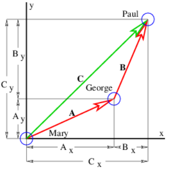
Figure 2.1.1: shows some examples of displacement vectors, i. e., vectors which represent the displacement of one object from another, and introduces the idea of vector addition. The tail of vector B is collocated with the head of vector A, and the vector which stretches from the tail of A to the head of B is the sum of A and B, called C in Figure 2.1.1:.
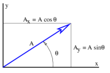
The quantities Ax,Ay etc., represent the Cartesian components of the vectors in Figure 2.1.1:. A vector can be represented either by its Cartesian components, which are just the projections of the vector onto the Cartesian coordinate axes, or by its direction and magnitude. The direction of a vector in two dimensions is generally represented by the counterclockwise angle of the vector relative to the x axis, as shown in Figure 2.1.2:. Conversion from one form to the other is given by the equations
A=(A2x+A2y)1/2θ=tan−1(Ay/Ax)
Ax=Acos(θ)Ay=Asin(θ)
where A is the magnitude of the vector. A vector magnitude is sometimes represented by absolute value notation: A ≡|A|.
Notice that the inverse tangent gives a result which is ambiguous relative to adding or subtracting integer multiples of π. Thus the quadrant in which the angle lies must be resolved by independently examining the signs of Ax and Ay and choosing the appropriate value of θ.
To add two vectors, A and B, it is easiest to convert them to Cartesian component form. The components of the sum C = A + B are then just the sums of the components:
Cx=Ax+BxCy=Ay+By
Subtraction of vectors is done similarly, e. g., if A = C - B, then
Ax=Cx−BxAy=Cy−By
A unit vector is a vector of unit length. One can always construct a unit vector from an ordinary (non-zero) vector by dividing the vector by its length: n = A∕|A|. This division operation is carried out by dividing each of the vector components by the number in the denominator. Alternatively, if the vector is expressed in terms of length and direction, the magnitude of the vector is divided by the denominator and the direction is unchanged.
Unit vectors can be used to define a Cartesian coordinate system. Conventionally, i, j, and k indicate the x, y, and z axes of such a system. Note that i, j, and k are mutually perpendicular. Any vector can be represented in terms of unit vectors and its Cartesian components: A = Axi + Ayj + Azk. An alternate way to represent a vector is as a list of components: A = (Ax,Ay,Az). We tend to use the latter representation since it is somewhat more economical notation.
There are two ways to multiply two vectors, yielding respectively what are known as the dot product and the cross product. The cross product yields another vector while the dot product yields a number. Here we will discuss only the dot product. The cross product will be presented later when it is needed.
Given vectors A and B, the dot product of the two is defined as
A⋅B≡|A‖B|cosθ
where θ is the angle between the two vectors. In two dimensions an alternate expression for the dot product exists in terms of the Cartesian components of the vectors:
A⋅B=AxBx+AyBy
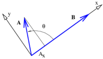
It is easy to show that this is equivalent to the cosine form of the dot product when the x axis lies along one of the vectors, as in Figure 2.1.3:. Notice in particular that Ax = |A| cos θ, while Bx = |B| and By = 0. Thus, A ⋅ B = |A| cos θ|B| in this case, which is identical to the form given in equation (2.5).
All that remains to be proven for Equation ??? to hold in general is to show that it yields the same answer regardless of how the Cartesian coordinate system is oriented relative to the vectors. To do this, we must show that AxBx + AyBy = Ax′Bx′ + Ay′By′, where the primes indicate components in a coordinate system rotated from the original coordinate system.
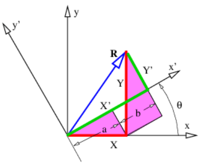
Figure 2.1.4: shows the vector R resolved in two coordinate systems rotated with respect to each other. From this figure it is clear that X′=a+b. Focusing on the shaded triangles, we see that a=Xcosθ and b=Ysinθ. Thus, we find X′=Xcosθ+Ysinθ. Similar reasoning shows that Y′=−Xsinθ+Ycosθ. Substituting these and using the trigonometric identity cos 2θ + sin 2θ = 1 results in
A′xB′x+A′yB′y=(Axcosθ+Aysinθ)(Bxcosθ+Bysinθ)+(−Axsinθ+Aycosθ)(−Bxsinθ+Bycosθ)=AxBx+AyBy
thus proving the complete equivalence of the two forms of the dot product as given by equations (2.5) and (2.6). Multiply out the above expression to verify this.
A numerical quantity that doesn’t depend on which coordinate system is being used is called a scalar. The dot product of two vectors is a scalar. However, the components of a vector, taken individually, are not scalars, since the components change as the coordinate system changes. Since the laws of physics cannot depend on the choice of coordinate system being used, we insist that physical laws be expressed in terms of scalars and vectors, but not in terms of the components of vectors.
In three dimensions the cosine form of the dot product remains the same, while the component form is
A⋅B=AxBx+AyBy+AzBz