2.2: Plane Waves

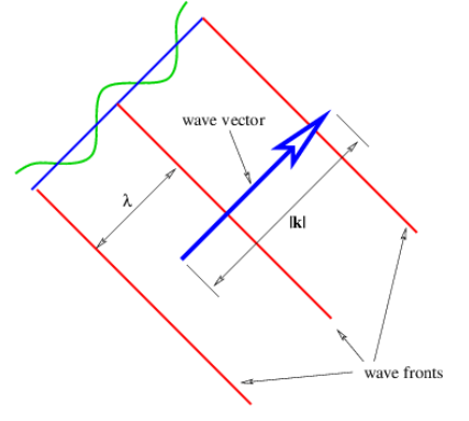
A plane wave in two or three dimensions is like a sine wave in one dimension except that crests and troughs aren’t points, but form lines (2-D) or planes (3-D) perpendicular to the direction of wave propagation. Figure \(\PageIndex{1}\) shows a plane sine wave in two dimensions. The large arrow is a vector called the wave vector, which defines (1) the direction of wave propagation by its orientation perpendicular to the wave fronts, and (2) the wavenumber by its length.

Figure \(\PageIndex{1}\): Definition sketch for a plane sine wave in two dimensions. The wave fronts are constant phase surfaces separated by one wavelength. The wave vector is normal to the wave fronts and its length is the wavenumber.

We can think of a wave front as a line along the crest of the wave. The equation for the displacement associated with a plane sine wave (of unit amplitude) in three dimensions at some instant in time is

\[h(x, y, z)=\sin (\mathbf{k} \cdot \mathbf{x})=\sin \left(k_{x} x+k_{y} y+k_{z} z\right)\label{2.9}\]

Since wave fronts are lines or surfaces of constant phase, the equation defining a wave front is simply \(\mathbf{k} \cdot \mathbf{x}=\text { const. }\)

In the two dimensional case we simply set k_z = 0. Therefore, a wave front, or line of constant phase ϕ in two dimensions is defined by the equation

\[\mathbf{k} \cdot \mathbf{x}=k_{x} x+k_{y} y=\phi \quad \text { (two dimensions). }\label{2.10}\]

This can be easily solved for y to obtain the slope and intercept of the wave front in two dimensions.

As for one dimensional waves, the time evolution of the wave is obtained by adding a term -ωt to the phase of the wave. In three dimensions the wave displacement as a function of both space and time is given by

\[h(x, y, z, t)=\sin \left(k_{x} x+k_{y} y+k_{z} z-\omega t\right)\label{2.11}\]

The frequency depends in general on all three components of the wave vector. The form of this function, \(\omega=\omega\left(k_{x}, k_{y} k_{z}\right)\) which as in the one dimensional case is called the dispersion relation, contains information about the physical behavior of the wave.

Some examples of dispersion relations for waves in two dimensions are as follows:

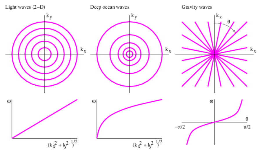
• Light waves in a vacuum in two dimensions obey \[\omega=c\left(k_{x}^{2}+k_{y}^{2}\right)^{1 / 2}\label{2.12}\] where c is the speed of light in a vacuum.
• Deep water ocean waves in two dimensions obey \[\omega=g^{1 / 2}\left(k_{x}^{2}+k_{y}^{2}\right)^{1 / 4} \quad \text { (ocean waves) }\label{2.13}\] where g is the strength of the Earth’s gravitational field as before.
• Certain kinds of atmospheric waves confined to a vertical x-z plane called gravity waves (not to be confused with the gravitational waves of general relativity) obey \[\omega=\frac{N k_{x}}{k_{z}} \quad \text { (gravity waves), }\label{2.14}\] where N is a constant with the dimensions of inverse time called the Brunt-Väisälä frequency.

Contour plots of these dispersion relations are plotted in the upper panels of figure 2.6. These plots are to be interpreted like topographic maps, where the lines represent contours of constant elevation. In the case of figure 2.6, constant values of frequency are represented instead. For simplicity, the actual values of frequency are not labeled on the contour plots, but are represented in the graphs in the lower panels. This is possible because frequency depends only on wave vector magnitude (k_x² + k _y²)^1∕2 for the first two examples, and only on wave vector direction θ for the third.

Figure \(\PageIndex{2}\): .6: Contour plots of the dispersion relations for three kinds of waves in two dimensions. In the upper panels the curves show lines or contours along which the frequency ω takes on constant values. Contours are drawn for equally spaced values of ω. For light and ocean waves the frequency depends only on the magnitude of the wave vector, whereas for gravity waves it depends only on the wave vector’s direction, as defined by the angle θ in the upper right panel. These dependences for each wave type are illustrated in the lower panels.