Physics LibreTexts

4.11: The Second Law of Thermodynamics (Answer)

  • Page ID
    10247
  • \( \newcommand{\vecs}[1]{\overset { \scriptstyle \rightharpoonup} {\mathbf{#1}} } \)

    \( \newcommand{\vecd}[1]{\overset{-\!-\!\rightharpoonup}{\vphantom{a}\smash {#1}}} \)

    \( \newcommand{\id}{\mathrm{id}}\) \( \newcommand{\Span}{\mathrm{span}}\)

    ( \newcommand{\kernel}{\mathrm{null}\,}\) \( \newcommand{\range}{\mathrm{range}\,}\)

    \( \newcommand{\RealPart}{\mathrm{Re}}\) \( \newcommand{\ImaginaryPart}{\mathrm{Im}}\)

    \( \newcommand{\Argument}{\mathrm{Arg}}\) \( \newcommand{\norm}[1]{\| #1 \|}\)

    \( \newcommand{\inner}[2]{\langle #1, #2 \rangle}\)

    \( \newcommand{\Span}{\mathrm{span}}\)

    \( \newcommand{\id}{\mathrm{id}}\)

    \( \newcommand{\Span}{\mathrm{span}}\)

    \( \newcommand{\kernel}{\mathrm{null}\,}\)

    \( \newcommand{\range}{\mathrm{range}\,}\)

    \( \newcommand{\RealPart}{\mathrm{Re}}\)

    \( \newcommand{\ImaginaryPart}{\mathrm{Im}}\)

    \( \newcommand{\Argument}{\mathrm{Arg}}\)

    \( \newcommand{\norm}[1]{\| #1 \|}\)

    \( \newcommand{\inner}[2]{\langle #1, #2 \rangle}\)

    \( \newcommand{\Span}{\mathrm{span}}\) \( \newcommand{\AA}{\unicode[.8,0]{x212B}}\)

    \( \newcommand{\vectorA}[1]{\vec{#1}}      % arrow\)

    \( \newcommand{\vectorAt}[1]{\vec{\text{#1}}}      % arrow\)

    \( \newcommand{\vectorB}[1]{\overset { \scriptstyle \rightharpoonup} {\mathbf{#1}} } \)

    \( \newcommand{\vectorC}[1]{\textbf{#1}} \)

    \( \newcommand{\vectorD}[1]{\overrightarrow{#1}} \)

    \( \newcommand{\vectorDt}[1]{\overrightarrow{\text{#1}}} \)

    \( \newcommand{\vectE}[1]{\overset{-\!-\!\rightharpoonup}{\vphantom{a}\smash{\mathbf {#1}}}} \)

    \( \newcommand{\vecs}[1]{\overset { \scriptstyle \rightharpoonup} {\mathbf{#1}} } \)

    \( \newcommand{\vecd}[1]{\overset{-\!-\!\rightharpoonup}{\vphantom{a}\smash {#1}}} \)

    \(\newcommand{\avec}{\mathbf a}\) \(\newcommand{\bvec}{\mathbf b}\) \(\newcommand{\cvec}{\mathbf c}\) \(\newcommand{\dvec}{\mathbf d}\) \(\newcommand{\dtil}{\widetilde{\mathbf d}}\) \(\newcommand{\evec}{\mathbf e}\) \(\newcommand{\fvec}{\mathbf f}\) \(\newcommand{\nvec}{\mathbf n}\) \(\newcommand{\pvec}{\mathbf p}\) \(\newcommand{\qvec}{\mathbf q}\) \(\newcommand{\svec}{\mathbf s}\) \(\newcommand{\tvec}{\mathbf t}\) \(\newcommand{\uvec}{\mathbf u}\) \(\newcommand{\vvec}{\mathbf v}\) \(\newcommand{\wvec}{\mathbf w}\) \(\newcommand{\xvec}{\mathbf x}\) \(\newcommand{\yvec}{\mathbf y}\) \(\newcommand{\zvec}{\mathbf z}\) \(\newcommand{\rvec}{\mathbf r}\) \(\newcommand{\mvec}{\mathbf m}\) \(\newcommand{\zerovec}{\mathbf 0}\) \(\newcommand{\onevec}{\mathbf 1}\) \(\newcommand{\real}{\mathbb R}\) \(\newcommand{\twovec}[2]{\left[\begin{array}{r}#1 \\ #2 \end{array}\right]}\) \(\newcommand{\ctwovec}[2]{\left[\begin{array}{c}#1 \\ #2 \end{array}\right]}\) \(\newcommand{\threevec}[3]{\left[\begin{array}{r}#1 \\ #2 \\ #3 \end{array}\right]}\) \(\newcommand{\cthreevec}[3]{\left[\begin{array}{c}#1 \\ #2 \\ #3 \end{array}\right]}\) \(\newcommand{\fourvec}[4]{\left[\begin{array}{r}#1 \\ #2 \\ #3 \\ #4 \end{array}\right]}\) \(\newcommand{\cfourvec}[4]{\left[\begin{array}{c}#1 \\ #2 \\ #3 \\ #4 \end{array}\right]}\) \(\newcommand{\fivevec}[5]{\left[\begin{array}{r}#1 \\ #2 \\ #3 \\ #4 \\ #5 \\ \end{array}\right]}\) \(\newcommand{\cfivevec}[5]{\left[\begin{array}{c}#1 \\ #2 \\ #3 \\ #4 \\ #5 \\ \end{array}\right]}\) \(\newcommand{\mattwo}[4]{\left[\begin{array}{rr}#1 \amp #2 \\ #3 \amp #4 \\ \end{array}\right]}\) \(\newcommand{\laspan}[1]{\text{Span}\{#1\}}\) \(\newcommand{\bcal}{\cal B}\) \(\newcommand{\ccal}{\cal C}\) \(\newcommand{\scal}{\cal S}\) \(\newcommand{\wcal}{\cal W}\) \(\newcommand{\ecal}{\cal E}\) \(\newcommand{\coords}[2]{\left\{#1\right\}_{#2}}\) \(\newcommand{\gray}[1]{\color{gray}{#1}}\) \(\newcommand{\lgray}[1]{\color{lightgray}{#1}}\) \(\newcommand{\rank}{\operatorname{rank}}\) \(\newcommand{\row}{\text{Row}}\) \(\newcommand{\col}{\text{Col}}\) \(\renewcommand{\row}{\text{Row}}\) \(\newcommand{\nul}{\text{Nul}}\) \(\newcommand{\var}{\text{Var}}\) \(\newcommand{\corr}{\text{corr}}\) \(\newcommand{\len}[1]{\left|#1\right|}\) \(\newcommand{\bbar}{\overline{\bvec}}\) \(\newcommand{\bhat}{\widehat{\bvec}}\) \(\newcommand{\bperp}{\bvec^\perp}\) \(\newcommand{\xhat}{\widehat{\xvec}}\) \(\newcommand{\vhat}{\widehat{\vvec}}\) \(\newcommand{\uhat}{\widehat{\uvec}}\) \(\newcommand{\what}{\widehat{\wvec}}\) \(\newcommand{\Sighat}{\widehat{\Sigma}}\) \(\newcommand{\lt}{<}\) \(\newcommand{\gt}{>}\) \(\newcommand{\amp}{&}\) \(\definecolor{fillinmathshade}{gray}{0.9}\)

    Check Your Understanding

    4.1. A perfect heat engine would have \(\displaystyle Q_c=0\), which would lead to \(\displaystyle e=1−Q_c/Q_h=1\). A perfect refrigerator would need zero work, that is, \(\displaystyle W=0\), which leads to \(\displaystyle K_R=Q_c/W→∞\).

    4.2. From the engine on the right, we have \(\displaystyle W=Q′_h−Q′_c\). From the refrigerator on the right, we have \(\displaystyle Q_h=Q_c+W\). Thus, \(\displaystyle W=Q′_h−Q′_c=Q_h−Q_c\).

    4.3. a. \(\displaystyle e=1−T_c/T_h=0.55\);

    b. \(\displaystyle Q_h=eW=9.1J\);

    c. \(\displaystyle Q_c=Q_h−W=4.1J\);

    d. \(\displaystyle −273°C\) and \(\displaystyle 400°C\)

    4.4. a. \(\displaystyle K_R=T_c/(T_h−T_c)=10.9\);

    b. \(\displaystyle Q_c=K_RW=2.18kJ\);

    c. \(\displaystyle Q_h=Q_c+W=2.38kJ\)

    4.5. When heat flows from the reservoir to the ice, the internal (mainly kinetic) energy of the ice goes up, resulting in a higher average speed and thus an average greater position variance of the molecules in the ice. The reservoir does become more ordered, but due to its much larger amount of molecules, it does not offset the change in entropy in the system.

    4.6. \(\displaystyle −Q/T_h; Q/T_c\); and \(\displaystyle Q(T_h−T_c)/(T_hT_c)\)

    4.7. a. 4.71 J/K;

    b. −4.18 J/K;

    c. 0.53 J/K

    Conceptual Questions

    1. Some possible solutions are frictionless movement; restrained compression or expansion; energy transfer as heat due to infinitesimal temperature nonuniformity; electric current flow through a zero resistance; restrained chemical reaction; and mixing of two samples of the same substance at the same state.

    3. The temperature increases since the heat output behind the refrigerator is greater than the cooling from the inside of the refrigerator.

    5. If we combine a perfect engine and a real refrigerator with the engine converting heat Q from the hot reservoir into work \(\displaystyle W=Q\) to drive the refrigerator, then the heat dumped to the hot reservoir by the refrigerator will be \(\displaystyle W+ΔQ\), resulting in a perfect refrigerator transferring heat \(\displaystyle ΔQ\) from the cold reservoir to hot reservoir without any other effect.

    7. Heat pumps can efficiently extract heat from the ground to heat on cooler days or pull heat out of the house on warmer days. The disadvantage of heat pumps are that they are more costly than alternatives, require maintenance, and will not work efficiently when temperature differences between the inside and outside are very large. Electric heating is much cheaper to purchase than a heat pump; however, it may be more costly to run depending on the electric rates and amount of usage.

    9. A nuclear reactor needs to have a lower temperature to operate, so its efficiency will not be as great as a fossil-fuel plant. This argument does not take into consideration the amount of energy per reaction: Nuclear power has a far greater energy output than fossil fuels.

    11. In order to increase the efficiency, the temperature of the hot reservoir should be raised, and the cold reservoir should be lowered as much as possible. This can be seen in Equation 4.3.

    13. adiabatic and isothermal processes

    15. Entropy will not change if it is a reversible transition but will change if the process is irreversible.

    17. Entropy is a function of disorder, so all the answers apply here as well.

    Problems

    19. \(\displaystyle 11.0×10^3 J\)

    21. \(\displaystyle 4.5pV_0\)

    23. 0.667

    25. a. 0.200;

    b. 25.0 J

    27. a. 0.67;

    b. 75 J;

    c. 25 J

    29. a. 600 J;

    b. 800 J

    31. a. 69 J;

    b. 11 J

    33. 2.0

    35. 50 J

    37.
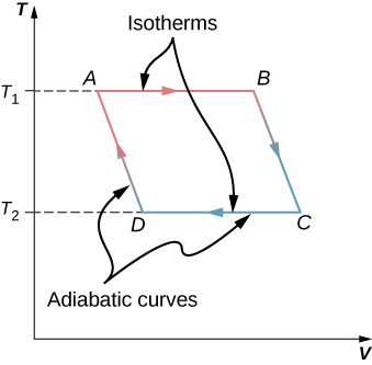
    The graph shows isotherms and adiabatic curves for Carnot cycle with four points A, B, C and D. The x-axis is V and y-axis is T. The value of T at A and B is T subscript 1 and at C and D is T subscript 2.

    39. a. 381 J;

    b. 619 J

    41. a. 546 K;

    b. 137 K

    43. –1 J/K

    45. –13 J(K mole)

    47. \(\displaystyle −\frac{Q}{T_h},\frac{Q}{T_c},Q(\frac{1}{T_c}−\frac{1}{T_h})\)

    49. a. –709 J/K;

    b. 1300 J/K;

    c. 591 J/K

    51. a. \(\displaystyle Q=nRΔT\);

    b. \(\displaystyle S=nRln(T_2/T_1)\)

    53. \(\displaystyle 3.78×10^{−3}W/K\)

    55. 430 J/K

    57. \(\displaystyle 80°C, 80°C, 6.70×10^4J\), 215 J/K, –190 J/K, 25 J/K

    59. \(\displaystyle ΔS_{H2O}=215J/K, ΔS_R=−208J/K, ΔS_U=7J/K\)

    61. a. 1200 J;

    b. 600 J;

    c. 600 J;

    d. 0.50

    63. \(\displaystyle ΔS=nC_Vln(\frac{T_2}{T_1})+nC_pln(\frac{T_3}{T_2})\)

    65. a. 0.33, 0.39;

    b. 0.91

    Additional Problems

    67. \(\displaystyle 1.45×10^7J\)

    69. a. \(\displaystyle V_B=0.042m^3,V_D=0.018m^3\);

    b. 13,000 J;

    c. 13,000 J;

    d. –8,000 J;

    e. –8,000 J;

    f. 6200 J;

    g. –6200 J;

    h. 39%; with temperatures efficiency is 40%, which is off likely by rounding errors.

    71. –670 J/K

    73. a. –570 J/K;

    b. 570 J/K

    75. 82 J/K

    77. a. 2000 J;

    b. 40%

    79. 60%

    81. 64.4%

    Challenge Problems

    83. derive

    85.derive

    87. 18 J/K

    89. proof

    91. \(\displaystyle K_R=\frac{3(p_1−p_2)V_1}{5p_2V_3−3p_1V_1−p_2V_1}\)

    93. \(\displaystyle W=110,000J\)

    Contributors and Attributions

    Samuel J. Ling (Truman State University), Jeff Sanny (Loyola Marymount University), and Bill Moebs with many contributing authors. This work is licensed by OpenStax University Physics under a Creative Commons Attribution License (by 4.0).


    This page titled 4.11: The Second Law of Thermodynamics (Answer) is shared under a CC BY 4.0 license and was authored, remixed, and/or curated by OpenStax via source content that was edited to the style and standards of the LibreTexts platform.