2.1: Damped Oscillators

Consider first the free oscillation of a damped oscillator. This could be, for example, a system of a block attached to a spring, like that shown in Figure \( 1.1\), but with the whole system immersed in a viscous fluid. Then in addition to the restoring force from the spring, the block experiences a frictional force. For small velocities, the frictional force can be taken to have the form \[-m \Gamma v ,\]

where \(\Gamma\) is a constant. Notice that because we have extracted the factor of the mass of the block in (2.1), \(1 / \Gamma\) has the dimensions of time. We can write the equation of motion of the system as \[\frac{d^{2}}{d t^{2}} x(t)+\Gamma \frac{d}{d t} x(t)+\omega_{0}^{2} x(t)=0 ,\]

where \(\omega_{0}=\sqrt{K / m}\). This equation is linear and time translation invariant, like the undamped equation of motion. In fact, it is just the form that we analyzed in the previous chapter, in (1.16). As before, we allow for the possibility of complex solutions to the same equation, \[\frac{d^{2}}{d t^{2}} z(t)+\Gamma \frac{d}{d t} z(t)+\omega_{0}^{2} z(t)=0 .\]

Because (1.71) is satisfied, we know from the arguments of of chapter 1 that we can find irreducible solutions of the form \[z(t)=e^{\alpha t} ,\]

where \(\alpha\) (Greek letter alpha) is a constant. Putting (2.4) into (2.2), we find \[\left(\alpha^{2}+\Gamma \alpha+\omega_{0}^{2}\right) e^{\alpha t}=0 .\]

Because the exponential never vanishes, the quantity in parentheses must be zero, thus \[\alpha=-\frac{\Gamma}{2} \pm \sqrt{\frac{\Gamma^{2}}{4}-\omega_{0}^{2}} .\]

From (2.6), we see that there are three regions for \(\Gamma\) compared to \(\omega_{0}\) that lead to different physics.

Overdamped Oscillators

If \(\Gamma / 2>\omega_{0}\), both solutions for \(\alpha\) are real and negative. The solution to (2.2) is a sum of decreasing exponentials. Any initial displacement of the system dies away with no oscillation. This is an overdamped oscillator.

The general solution in the overdamped case has the form, \[x(t)=z(t)=A_{+} e^{-\Gamma_{+} t}+A_{-} e^{-\Gamma_{-} t},\]

where \[\Gamma_{\pm}=\frac{\Gamma}{2} \pm \sqrt{\frac{\Gamma^{2}}{1}-\omega_{0}^{2}} .\]

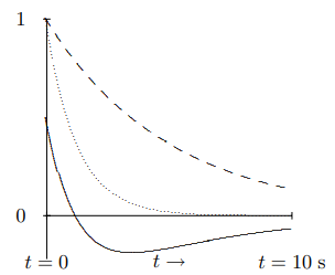
Figure \( 2.1\): Solutions to the equation of motion for an overdamped oscillator.

An example is shown in Figure \( 2.1\). The dotted line is \(e^{-\Gamma+t}\) for \(\Gamma = 1 s^{-1}\) and \(\omega_{0}=.4 \mathrm{~s}^{-1}\). The dashed line is \(e^{-\Gamma_{-} t}\). The solid line is a linear combination, \(e^{-\Gamma_{+} t}-\frac{1}{2} e^{-\Gamma_{-} t}\).

In the overdamped situation, there is really no oscillation. If the mass is initially moving very fast toward the equilibrium position, it can overshoot, as shown in Figure \( 2.1\). However, it then moves exponentially back toward the equilibrium position, without ever crossing the equilibrium value of the displacement a second time. Thus in the free motion of an overdamped oscillator, the equilibrium position is crossed either zero or one times.

Underdamped Oscillators

If \(\Gamma / 2<\omega_{0}\), the expression inside the square root is negative, and the solutions for \(\alpha\) are a complex conjugate pair, with negative real part. Thus the solutions are products of a decreasing exponential, \(e^{-\Gamma t / 2}\), times complex exponentials (or sines and cosines) \(e^{\pm i \omega t}\), where \[\omega^{2}=\omega_{0}^{2}-\Gamma^{2} / 4 .\]

This is an underdamped oscillator.

Most of the systems that we think of as oscillators are underdamped. For example, a system of a child sitting still on a playground swing is an underdamped pendulum that can oscillate many times before frictional forces bring it to rest.

The decaying exponential \(e^{-\Gamma t / 2} e^{-i(\omega t-\theta)}\) spirals in toward the origin in the complex plane. Its real part, \(e^{-\Gamma t / 2} \cos (\omega t-\theta)\), describes a function that oscillates with decreasing amplitude. In real form, the general solution for the underdamped case has the form, \[x(t)=A e^{-\Gamma t / 2} \cos (\omega t-\theta),\]

or \[x(t)=e^{-\Gamma t / 2}(c \cos (\omega t)+d \sin (\omega t)),\]

where \(A\) and \(\omega\) are related to \(c\) and \(d\) by (1.97) and (1.98). This is shown in Figure \( 2.2\) (to be compared with Figure \( 1.9\)). The upper figure shows the complex plane with \(e^{-\Gamma t / 2} e^{-i(\omega t-\theta)}\) plotted for equally spaced values of \(t\). The lower figure is the real part, \(\cos (\omega t-\theta) \rightarrow\), for the same values of \(t\) plotted versus \(t\). In the underdamped case, the equilibrium position is crossed an infinite number of times, although with exponentially decreasing amplitude!

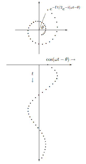
Figure \( 2.2\): A damped complex exponential.

Critically Damped Oscillators

If \(\Gamma / 2=\omega_{0}\), then (2.4), gives only one solution, \(e^{-\Gamma t / 2}\). We know that there will be two solutions to the second order differential equation, (2.2). One way to find the other solution is to approach this situation from the underdamped case as a limit. If we write the solutions to the underdamped case in real form, they are \(e^{-\Gamma t / 2} \cos \omega t\) and \(e^{-\Gamma t / 2} \sin \omega t\). Taking the limit of the first as \(\omega \rightarrow 0\) gives \(e^{-\Gamma t / 2}\), the solution we already know. Taking the limit of the second gives 0. However, if we first divide the second solution by \(\omega\), it is still a solution because \(\omega\) does not depend on \(t\). Now we can get a nonzero limit: \[\lim _{\omega \rightarrow 0} \frac{1}{\omega} e^{-\Gamma t / 2} \sin \omega t=t e^{-\Gamma t / 2} .\]

Thus \(t e^{-\Gamma t / 2}\) is also a solution. You can also check this explicitly, by inserting it back into (2.2). This is called the critically damped case because it is the boundary between overdamping and underdamping.

A familiar system that is close to critical damping is the combination of springs and shock absorbers in an automobile. Here the damping must be large enough to prevent the car from bouncing. But if the damping from the shocks is too high, the car will not be able to respond quickly to bumps and the ride will be rough.

The general solution in the critically damped case is thus \[c e^{-\Gamma t / 2}+d t e^{-\Gamma t / 2} .\]

This is illustrated in Figure \( 2.3\). The dotted line is \(e^{-\Gamma t}\) for \(\Gamma=1 \mathrm{~s}^{-1}\). The dashed line is \(t e^{-\Gamma t}\). The solid line is a linear combination, \((1-t) e^{-\Gamma t}\).

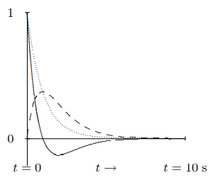
Figure \( 2.3\): Solutions to the equation of motion for a critically damped oscillator.

As in the overdamped situation, there is no real oscillation for critical damping. However, again, the mass can overshoot and then go smoothly back toward the equilibrium position, without ever crossing the equilibrium value of the displacement a second time. As for overdamping, the equilibrium position is crossed either once or not at all.