2.3: Resonance

The \(\left(\omega_{0}^{2}-\omega_{d}^{2}\right)^{2}\) term in the denominator of (2.22) goes to zero for \(\omega_{d} = \omega_{0}\). If the damping is small, this behavior of the denominator gives rise to a huge increase in the response of the system to the driving force at \(\omega_{d} = \omega_{0}\). The phenomenon is called resonance. The angular frequency \(\omega_{0}\) is the resonant angular frequency. When \(\omega_{d} = \omega_{0}\), the system is said to be “on resonance”.

The phenomenon of resonance is both familiar and spectacularly important. It is familiar in situations as simple as building up a large amplitude in a child’s swing by supplying a small force at the same time in each cycle. Yet simple as it is, it is crucial in many devices and many delicate experiments in physics. Resonance phenomena are used ubiquitously to build up a large, measurable response to a very small disturbance.

Very often, we will ignore damping in forced oscillations. Near a resonance, this is not a good idea, because the amplitude, (2.22), goes to infinity as \(\Gamma \rightarrow 0\) for \(\omega_{d} = \omega_{0}\). Infinities are not physical. This infinity never occurs in practice. One of two things happen before the amplitude blows up. Either the damping eventually cannot be ignored, so the response looks like (2.22) for nonzero \(\Gamma\), or the amplitude gets so large that the nonlinearities in the system cannot be ignored, so the equation of motion no longer looks like (2.16).

Work

It is instructive to consider the work done by the external force in (2.16). To do this we must use the real force, (2.14), and the real displacement (2.25), rather than their complex extensions, because, unlike almost everything else we talk about, the work is a nonlinear function of the force. The power expended by the force is the product of the driving force and the velocity, \[P(t)=F(t) \frac{\partial}{\partial t} x(t)=-F_{0} \omega_{d} A \cos \omega_{d} t \sin \omega_{d} t+F_{0} \omega_{d} B \cos ^{2} \omega_{d} t .\]

The first term in (2.26) is proportional to \(\sin 2 \omega_{d} t\). Thus it is sometimes positive and sometimes negative. It averages to zero over any complete half-period of oscillation, a time \(\pi / \omega_{d}\), because \[\int_{t_{0}}^{l_{0}+\pi / \omega_{d}} d t \sin 2 \omega_{d} t=-\left.\frac{1}{2} \cos 2 \omega_{d} t\right|_{t_{0}} ^{t_{0}+\pi / \omega_{d}}=0 .\]

This is why \(A\) is called the elastic amplitude. If \(A\) dominates, then energy fed into the system at one time is returned at a later time, as in an elastic collision in mechanics.

The second term in (2.26), on the other hand, is always positive. It averages to \[P_{\text {average }}=\frac{1}{2} F_{0} \omega_{d} B .\]

This is why \(B\) is called the absorptive amplitude. It measures how fast energy is absorbed by the system. The absorbed power, \(P_{\text {average }\), reaches a maximum on resonance, at \(\omega_{0} = \omega_{d}\). This is a diagnostic that is often used to find resonances in experimental situations. Note that the dependence of \(B\) on \(\omega_{d}\) looks qualitatively similar to that of \(P_{\text {average }\), which is shown in Figure \( 2.5\) for \(\Gamma = \(\omega_{0} / 2\). However, they differ by a factor of \(\omega_{d}\). In particular, the maximum of \(B\) occurs slightly below resonance.

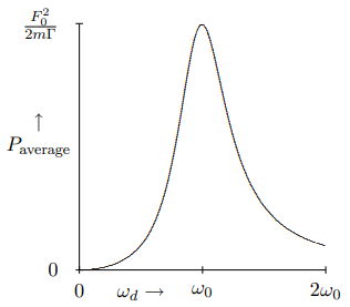
Figure \( 2.5\): The average power lost to the frictional force as a function of \(\omega_{d}\) for \(\Gamma=\omega_{0} / 2\).

Resonance Width and Lifetime

Both the height and the width of the resonance curve in Figure \( 2.5\) are determined by the frictional term, \(\Gamma\), in the equation of motion. The maximum average power is inversely proportional to \(\Gamma\), \[\frac{F_{0}^{2}}{2 m \Gamma} .\]

The width (for fixed height) is determined by the ratio of \(\Gamma\) to \(\omega_{0}\). In fact, you can check that the values of \(\omega_{d}\) for which the average power loss is half its maximum value are \[\omega_{1 / 2}=\sqrt{\omega_{0}^{2}+\frac{\Gamma^{2}}{4}} \pm \frac{\Gamma}{2} .\]

The \(\Gamma\) is the “full width at half-maximum” of the power curve. In Figure \( 2.6\) and Figure \( 2.7\), we show the average power as a function of \(\omega_{d}\) for \(\Gamma = \omega_{0} / 4\) and \(\Gamma = \omega_{0}\). The linear dependence of the width on \(\Gamma\) is clearly visible. The dotted lines show the position of half-maximum.

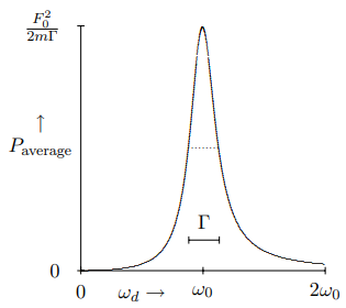
Figure \( 2.6\): The average power lost to the frictional force as a function of \(\omega_{d}\) for \(\Gamma = \omega_{0} / 4\).

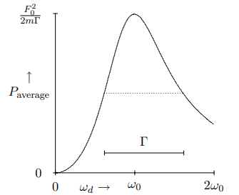
Figure \( 2.7\): The average power lost to the frictional force as a function of \(\omega_{d}\) for \(\Gamma = \omega_{0}\).

This relation is even more interesting in view of the relationship between \(\Gamma\) and the time dependence of the free oscillation. The lifetime of the state in free oscillation is of order \(1 / \Gamma\). In other words, the width of the resonance peak in forced oscillation is inversely proportional to the lifetime of the corresponding normal mode of free oscillation. This inverse relation is important in many fields of physics. An extreme example is particle physics, where very short-lived particles can be described as resonances. The quantum mechanical waves associated with these particles have angular frequencies proportional to their energies, \[E=\hbar \omega\]

where \(\hbar\) is Planck’s constant divided by \(2 \pi\), \[h \approx 6.626 \times 10^{-34} \mathrm{Js} .\]

The lifetimes of these particles, some as short as \(10^{-24}\) seconds, are far too short to measure directly. However, the short lifetime shows up in the large width of the distribution of energies of these states. That is how the lifetimes are actually inferred.

Phase Lag

We can also write (2.25) as \[x(t)=R \cos \left(\omega_{d} t-\theta\right)\)

for \[R=\sqrt{A^{2}+B^{2}}, \quad \theta=\arg (A+i B) .\]

The phase angle, \(\theta\), measures the phase lag between the external force and the system’s response. The actual time lag is \(\theta / \omega_{d}\). The displacement reaches its maximum a time \(\theta / \omega_{d}\) after the force reaches its maximum.

Note that as the frequency increases, \(\theta\) increases and the motion lags farther and farther behind the external force. The phase angle, \(\theta\), is determined by the relative importance of the restoring force and the inertia of the oscillator. At low frequencies (compared to \(\omega_{0}\)), inertia (an imprecise word for the \(ma\) term in the equation of motion) is almost irrelevant because things are moving very slowly, and the motion is very nearly in phase with the force. Far beyond resonance, the inertia dominates. The mass can no longer keep up with the restoring force and the motion is nearly \(180^{\circ}\) out of phase with the force. We will work out a detailed example of this in the next section.

The phase lag goes through \(\pi / 2\) at resonance, as shown in the graph in Figure \( 2.8\) for \(\Gamma = \omega_{0} / 2\). A phase lag of \(\pi / 2\) is another frequently used diagnostic for resonance.

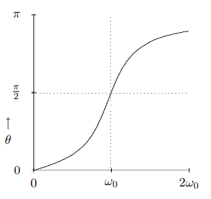
Figure \( 2.8\): A plot of the phase lag versus frequency in a damped forced oscillator.