2.2: Forced Oscillations

The damped oscillator with a harmonic driving force, has the equation of motion \[\frac{d^{2}}{d t^{2}} x(t)+\Gamma \frac{d}{d t} x(t)+\omega_{0}^{2} x(t)=F(t) / m ,\]

where the force is \[F(t)=F_{0} \cos \omega_{d} t .\]

The \(\omega_{d} / 2 \pi\) is called the driving frequency. Notice that it is not necessarily the same as the natural frequency, \(\omega_{0} / 2 \pi\), nor is it the oscillation frequency of the free system, (2.9). It is simply the frequency of the external force. It can be tuned completely independently of the other parameters of the system. It would be correct but awkward to refer to \(\omega_{d}\) as the driving angular frequency. We will simply call it the driving frequency, ignoring its angular character.

The angular frequencies, \(\omega_{d}\) and \(\omega_{0}\), appear in the equation of motion, (2.15), in completely different ways. You must keep the distinction in mind to understand forced oscillation. The natural angular frequency of the system, \(\omega_{0}\), is some combination of the masses and spring constants (or whatever relevant physical quantities determine the free oscillations). The angular frequency, \(\omega_{d}\), enters only through the time dependence of the driving force. This is the new aspect of forced oscillation. To exploit this new aspect fully, we will look for a solution to the equation of motion that oscillates with the same angular frequency, \(\omega_{d}\), as the driving force.

We can relate (2.14) to an equation of motion with a complex driving force \[\frac{d^{2}}{d t^{2}} z(t)+\Gamma \frac{d}{d t} z(t)+\omega_{0}^{2} z(t)=\mathcal{F}(t) / m ,\]

where \[\mathcal{F}(t)=F_{0} e^{-i \omega_{d} t} .\]

This works because the equation of motion, (2.14), does not involve \(i\) explicitly and because \[\operatorname{Re} \mathcal{F}(t)=F(t) .\]

If \(z(t)\) is a solution to (2.16), then you can prove that \(x(t)=\operatorname{Re} z(t)\) is a solution (2.14) by taking the real part of both sides of (2.16).

The advantage to the complex exponential force, in (2.16), is that it is irreducible, it behaves simply under time translations. In particular, we can find a steady state solution proportional to the driving force, \(e^{-i \omega_{d} t}\), whereas for the real driving force, the \(\cos \omega_{d} t\) and \(\sin \omega_{d} t\) forms get mixed up. That is, we look for a steady state solution of the form \[z(t)-\mathcal{A} e^{-i \omega_{d} t}\]

The steady state solution, (2.19), is a particular solution, not the most general solution to (2.16). As discussed in chapter 1, the most general solution of (2.16) is obtained by adding to the particular solution the most general solution for the free motion of the same oscillator (solutions of (2.3)). In general we will have to include these more general contributions to satisfy the initial conditions. However, as we have seen above, all of these solutions die away exponentially with time. They are what are called “transient” solutions. It is only the steady state solution that survives for a long time in the presence of damping. Unlike the solutions to the free equation of motion, the steady state solution has nothing to do with the initial values of the displacement and velocity. It is determined entirely by the driving force, (2.17). You will explore the transient solutions in problem (2.4).

Putting (2.19) and (2.17) into (2.16) and cancelling a factor of \(e^{-i \omega_{d} t}\) from each side of the resulting equation, we get \[\left(-\omega_{d}^{2}-i \Gamma \omega_{d}+\omega_{0}^{2}\right) \mathcal{A}=\frac{F_{0}}{m} ,\]

or \[\mathcal{A}=\frac{F_{0} / m}{\omega_{0}^{2}-i \Gamma \omega_{d}-\omega_{d}^{2}} .\]

Notice that we got the solution just using algebra. This is the advantage of starting with the irreducible solution, (2.19).

The amplitude, (2.21), of the displacement is proportional to the amplitude of the driving force. This is just what we expect from linearity (see problem (2.2)). But the coefficient of proportionality is complex. To see what it looks like explicitly, multiply the numerator and denominator of the right-hand side of (2.21) by \(\omega_{0}^{2}+i \Gamma \omega_{d}-\omega_{d}^{2}\), to get the complex numbers into the numerator \[\mathcal{A}=\frac{\left(\omega_{0}^{2}+i \Gamma \omega_{d}-\omega_{d}^{2}\right) F_{0} / m}{\left(\omega_{0}^{2}-\omega_{d}^{2}\right)^{2}+\Gamma^{2} \omega_{d}^{2}} .\]

The complex number \(\mathcal{A}\) can be written as \(A+i B\), with \(A\) and \(B\) real: \[A=\frac{\left(\omega_{0}^{2}-\omega_{d}^{2}\right) F_{0} / T n}{\left(\omega_{0}^{2}-\omega_{d}^{2}\right)^{2}+\Gamma^{2} \omega_{d}^{2}} ;\]

\[B=\frac{\Gamma \omega_{d} F_{0} / m}{\left(\omega_{0}^{2}-\omega_{d}^{2}\right)^{2}+\Gamma^{2} \omega_{d}^{2}}\]

Then the solution to the equation of motion for the real driving force, (2.14), is \[x(t)=\operatorname{Re} z(t)=\operatorname{Re}\left(\mathcal{A} e^{-i \omega_{d} t}\right)=A \cos \omega_{d} t+B \sin \omega_{d} t .\]

Thus the solution for the real force is a sum of two terms. The term proportional to \(A\) is in phase with the driving force (or \(180^{\circ}\) out of phase), while the term proportional to \(B\) is \(90^{\circ}\) out of phase. The advantage of going to the complex driving force is that it allows us to get both at once. The coefficients, \(A\) and \(B\), are shown in the graph in Figure \( 2.4\) for \(\Gamma=\omega_{0} / 2\).

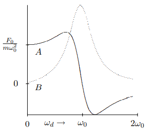
Figure \( 2.4\): The elastic and absorptive amplitudes, plotted versus \(\omega_{d}\). The absorptive amplitude is the dotted line.

The real part of \(\mathcal{A},\), \(A=\operatorname{Re} \mathcal{A}), is called the elastic amplitude and the imaginary part of \(\mathcal{A}\), \(B=\operatorname{Im} \mathcal{A}\), is called the absorptive amplitude. The reason for these names will become apparent below, when we consider the work done by the driving force.