3.1: More than One Degree of Freedom

In general, the number of degrees of freedom of a system is the number of independent coordinates required to specify the system’s configuration. The more degrees of freedom the system has, the larger the number of independent ways that the system can move. The more possible motions, you might think, the more complicated the system will be to analyze. In fact, however, using the tools of linear algebra, we will see that we can deal with systems with many degrees of freedom in a straightforward way.

Coupled Oscillators

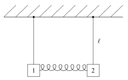
Figure \( 3.1\): Two pendulums coupled by a spring.

Consider the system of two pendulums shown in Figure \( 3.1\). The pendulums consist of rigid rods pivoted at the top so they oscillate without friction in the plane of the paper. The masses at the ends of the rods are coupled by a spring. We will consider the free motion of the system, with no external forces other than gravity. This is a classic example of two “coupled oscillators.” The spring that connects the two oscillators is the coupling. We will assume that the spring in Figure \( 3.1\) is unstretched when the two pendulums are hanging straight down, as shown. Then the equilibrium configuration is that shown in Figure \( 3.1\). This is an example of a system with two degrees of freedom, because two quantities, the displacements of each of the two blocks from equilibrium, are required to specify the configuration of the system. For example, if the oscillations are small, we can specify the configuration by giving the horizontal displacement of each of the two blocks from the equilibrium position.

Suppose that block 1 has mass \(m_{1}\), block 2 has mass \(m_{2}\), both pendulums have length \(\ell\) and the spring constant is \(\kappa\) (Greek letter kappa). Label the (small) horizontal displacements of the blocks to the right, \(x_{1}\) and \(x_{2}\), as shown in Figure \( 3.2\). We could have called these

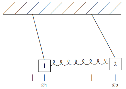
Figure \( 3.2\): Two pendulums coupled by a spring displaced from their equilibrium positions.

masses and displacements anything, but it is very convenient to use the same symbol, \(x\), with different subscripts. We can then write Newton’s law, \(F = m a\), in a compact and useful form. \[m_{j} \frac{d^{2}}{d t^{2}} x_{j}=F_{j} ,\]

for \(j\) = 1 to 2, where \(F_{1}\) is the horizontal force on block 1 and \(F_{2}\) is the horizontal force on block 2. Because there are two values of \(j\), (3.1) is two equations; one for \(j\) = 1 and another for \(j\) = 2. These are the two equations of motion for the system with two degrees of freedom. We will often refer to all the masses, displacements or forces at once as \(m_{j}\), \(x_{j}\) or \(F_{j}\), respectively. For example, we will say that \(F_{j}\) is the horizontal force on the \(j\)th block. This is an example of the use of “indices” (\(j\) is an index) to simplify the description of a system with more than one degree of freedom.

When the blocks move horizontally, they will move vertically as well, because the length of the pendulums remains fixed. Because the vertical displacement is second order in the \(x_{j}\)s, \[y_{j} \approx \frac{x_{j}^{2}}{2} ,\]

we can ignore it in thinking about the spring. The spring stays approximately horizontal for small oscillations.

To find the equation of motion for this system, we must find the forces, \(F_{j}\), in terms of the displacements, \(x_{j}\). It is the approximate linearity of the system that allows us to do this in a useful way. The forces produced by the Hooke’s law spring, and the horizontal forces on the pendulums due to the tension in the string (which in turn is due to gravity) are both approximately linear functions of the displacements for small displacements. Furthermore, the forces vanish when both the displacements vanish, because the system is in equilibrium. Thus each of the forces is some constant (different for each block) times \(x_{1}\) plus some other constant times \(x_{2}\). It is convenient to write this as follows: \[F_{1}=-K_{11} x_{1}-K_{12} x_{2}, \quad F_{2}=-K_{21} x_{1}-K_{22} x_{2} ,\]

or more compactly, \[F_{j}=-\sum_{k=1}^{2} K_{j k} x_{k}\]

for \(j\) = 1 to 2. We have written the four constants as \(K_{11}\), \(K_{12}\), \(K_{21}\) and \(K_{22}\) in order to write the force in this compact way. Later, we will call these constants the matrix elements of the \(K\) matrix. In this notation, the equations of motion are \[m_{j} \frac{d^{2}}{d t^{2}} x_{j}=-\sum_{k=1}^{2} K_{j k} x_{k}\]

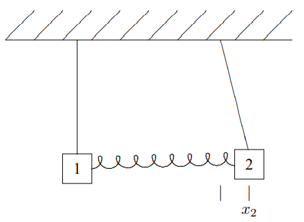
Figure \( 3.3\): Two pendulums coupled by a spring with block 2 displaced from an equilibrium position.

Because of the linearity of the system, we can find the constants, \(K_{jk}\), by considering the displacements of the blocks one at a time. Then we find the total force using (3.4). For example, suppose we displace block 2 with block 1 held fixed in its equilibrium position and look at the forces on both blocks. This will allow us to compute \(K_{12}\) and \(K_{22}\). The system with block two displaced is shown in Figure \( 3.3\). The forces on the blocks are shown in Figure \( 3.4\), where \(T_{j}\) is the tension in the \(j\)th pendulum string. \(F_{12}\) is the force on block 1 due to the displacement of block 2. \(F_{22}\) is the force on block 2 due to the displacement of block 2. For small displacements, the restoring force from the spring is nearly horizontal and equal to \(\kappa x_{2}\) on block 1 and \(-\kappa x_{2}\) on block 2. Likewise, in the limit of small displacement, the vertical component of the force from the tension \(T_{2}\) nearly cancels the gravitational force on block 2, \(m_{2}g\), so that the horizontal component of the tension gives a restoring force \(-x_{2} m_{2} g / \ell\) on block 2. For block 1, the force from the tension \(T_{1}\) just cancels the gravitational force \(m_{1}g\). Thus \[F_{12} \approx \kappa x_{2}, \quad F_{22} \approx-\frac{m_{2} g x_{2}}{\ell}-\kappa x_{2},\]

and \[K_{12} \approx-\kappa, \quad K_{22} \approx \frac{m_{2} g}{\ell}+\kappa .\]

An analogous argument shows that \[K_{21} \approx-\kappa, \quad K_{11} \approx \frac{m_{1} g}{\ell}+\kappa .\]

Notice that \[K_{12}=K_{21} .\]

We will see below that this is an example of a very general relation.

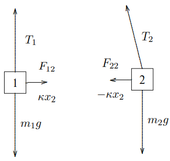
Figure \( 3.4\): The forces on the two blocks in Figure \( 3.3\).

Linearity and Normal Modes

3-1
We will see in this chapter that the most general possible motion of this system, and of any such system of oscillators, can be decomposed into particularly simple solutions, in which all the degrees of freedom oscillate with the same frequency. These simple solutions are called “normal modes.” The displacements for the most general motion can be written as sums of the simple solutions. We will study how this works in detail later, but it may be useful to see it first. A possible motion of the system of two coupled oscillators is animated in program 3-1. Below the actual motion, we show the two simple motions into which the more complicated motion can be decomposed. For this system, the normal mode with the lower frequency is one in which the displacements of the two blocks are the same: \[x_{1}(t)=x_{2}(t)=b_{1} \cos \left(\omega_{1} t-\theta_{1}\right) .\]

The other normal mode is one in which the displacements of the two blocks are opposite \[x_{1}(t)=-x_{2}(t)=b_{2} \cos \left(\omega_{2} t-\theta_{2}\right) .\]

The sum of these two simple motions gives the much more complicated motion shown in program 3-1.

\(n\) Coupled Oscillators

Before we try to solve the equations of motion, (3.5), let us generalize the discussion to systems with more degrees of freedom. Consider the oscillation of a system of \(n\) particles connected by various springs with no damping. Our analysis will be completely general, but for simplicity, we will talk about the particles as if they are constrained to move in the \(x\) direction, so that we can measure the displacement of the \(j\)th particle from equilibrium with the coordinate \(x_{j}\). Then the equilibrium configuration is the one in which all the \(x_{j}\)s are all zero.

Newton’s law, \(F = ma\), for the motion of the system gives \[m_{j} \frac{d^{2} x_{j}}{d t^{2}}=F_{j}\]

where \(m_{j}\) is the mass of the \(j\)th particle, \(F_{j}\) is the force on it. Because the system is linear, we expect that we can write the force as follows (as in (3.4)): \[F_{j}=-\sum_{k=1}^{n} K_{j k} x_{k}\]

for \(j = 1\) to \(n\). The constant, \(-K_{j k}\), is the force per unit displacement of the \(j\)th particle due to a displacement \(x_{k}\) of the \(k\)th particle. Note that all the \(F_{j}\)s vanish at equilibrium when all the \(x_{j}\)s are zero. Thus the equations of motion are \[m_{j} \frac{d^{2} x_{j}}{d t^{2}}=-\sum_{k} K_{j k} x_{k}\]

for \(j = 1\) to \(n\).

To measure \(K_{jk}\), make a small displacement, \(x_{k}\), of the \(k\)th particle, keeping all the other particles fixed at zero, assumed to be an equilibrium position. Then measure the force, \(F_{jk}\) on the \(j\)th particle with only the \(k\)th particle displaced. Since the system is linear (because it is made out of springs or in general, as long as the displacement is small enough), the force is proportional to the displacement, \(x_{k}\). The ratio of \(F_{jk}\) to \(x_{k}\) is \(-K_{jk}\): \[K_{j k}=-F_{j k} / x_{k} \text { when } x_{\ell}=0 \text { for } \ell \neq k .\]

Note that \(K_{jk}\) is defined with a \(-\) sign, so that a positive \(K\) is a force that is opposite to the displacement, and therefore tends to return the system to equilibrium.

Because the system is linear, the total force due to an arbitrary displacement is the sum of the contributions from each displacement. Thus \[F_{j}=\sum_{k} F_{j k}=-\sum_{k} K_{j k} x_{k}\]

Let us now try to understand (3.9). If we consider systems with no damping, the forces can be derived from a potential energy, \[F_{j}=-\frac{\partial V}{\partial x_{j}} .\]

But then by differentiating equation (3.16) we find that \[K_{j k}=\frac{\partial^{2} V}{\partial x_{j} \partial x_{k}} .\]

The partial differentiations commute with one another, thus equation (3.18) implies \[K_{j k}=K_{k j} .\]

In words, the force on particle \(j\) due to a displacement of particle \(k\) is equal to the force on particle \(k\) due to the displacement of particle \(j\).