3.3: Normal Modes

If there is only one degree of freedom, then both \(X\) and \(M^{-1}\) are just numbers and the solutions to the equation of motion, (3.62), have the form of a constant amplitude times an exponential factor. In fact, we saw that this form is related to a very general fact about the physics – time translation invariance, (1.33). The arguments of chapter 1, (1.71)-(1.85), did not depend on the number of degrees of freedom. Thus they show that here again, we can find irreducible solutions, that go into themselves up to an overall constant when the clocks are reset. As in chapter 1, the first step is to allow the solutions to be complex. That is, we replace (3.62) by \[\frac{d^{2} Z}{d t^{2}}=-M^{-1} K Z ,\]

where \(Z\) is a complex \(n\) vector with components, \(z_{j}\). The real parts of the components of \(Z\) are the components of a real solution satisfying (3.62), \[x_{j}=\operatorname{Re} z_{j} .\]

We will say that the real vector, \(X\), is the real part of the complex vector, \(Z\), \[X=\operatorname{Re} Z ,\]

if (3.64) is satisfied.

Just as in chapter 1, we know that we can find irreducible solutions that have the same form up to an overall constant when the clocks are reset. We know from (1.85) that these have the form \[Z(t)=A e^{-i \omega t}\]

where \(A\) is some constant \(n\)-vector and the angular frequency, \(\omega\), is still just a number. Now if \(t \rightarrow t + a\), \[Z(t) \rightarrow Z(t+a)=e^{=i \omega a} Z(t) .\)

While the irreducible form, (3.66), comes just from time translation invariance, we must still look at the equations of motion to determine the vector, \(A\) and the angular frequency, \(\omega\). Inserting (3.66) into (3.63), doing the differentiation and canceling the exponential factors from both sides, we find that (3.66) is a solution if \[\omega^{2} A=M^{-1} K A .\]

This matrix equation is an eigenvalue equation of the form that we discussed in (3.51)-(3.57). \(\omega^{2}\) is the eigenvalue of the matrix \(M^{-1}K\) and \(A\) is the corresponding eigenvector. Let us see what it means physically.

The real part of the column vector \(Z\) specifies the displacement of each of the degrees of freedom of the system. The eigenvalue equation, (3.68), does not involve any complex numbers (because we have not put in any damping). Therefore (as we will see explicitly below), we can choose the solutions so that all the components of \(A\) are real. Then the real part of the complex solutions we seek in (3.66) is \[X(t)=A \cos \omega t ,\]

or in terms of the components of \(A\), \[A=\left(\begin{array}{c}
a_{1} \\
a_{2} \\
\vdots
\end{array}\right) .\]

\[x_{1}(t)=a_{1} \cos \omega t, \quad x_{2}(t)=a_{2} \cos \omega t, \quad \text { etc. }\]

Not only does everything move with the same frequency, but the ratios of displacements of the individual degrees of freedom are fixed. Everything oscillates in phase. The only difference between the motion of the different degrees of freedom is their different amplitudes from the different components of \(A\).

The point is worth repeating. Time translation invariance and linearity imply that we can always find irreducible solutions, (3.67), in which all the degrees of freedom oscillate with the same frequency. The extra piece of information that leads to (3.69) is dynamical. If there is no damping, then all the components of \(A\) can be chosen to be real, and all the degrees of freedom oscillate not only with the same frequency, but also with the same phase.

If such a solution is to satisfy the equations of motion, then the acceleration must also be proportional to \(A\), so that the individual displacements don’t get out of synch. But that is what (3.68) is telling us. \(-M^{-1}K\) is the matrix that, acting on the displacement, gives the acceleration. The eigenvalue equation (3.68) means that the acceleration is proportional to \(A\) again. The constant of proportionality, \(\omega^{2}\), is the return force per unit displacement per unit mass for the particular displacement specified by \(A\).

We have already discussed the mathematical structure of the eigenvalue equation in (3.51)-(3.57). We will do it again, for emphasis, in the case of physical interest, (3.68). It should be clear that not every value of \(A\) and \(\omega^{2}\) gives a solution of (3.68). We will solve for the allowed values by first finding the possible values of \(\oemga^{2}\) and then finding the corresponding values of \(A\). To find the eigenvalues, note that (3.68) can be rewritten as \[\left[M^{-1} K-\omega^{2} I\right] A=0 ,\]

where \(I\) is the \(n \times n\) identity matrix. (3.72) is just a compact way of representing \(n\) homogeneous linear equations in the \(n\) components of \(A\) where the coefficients depend on \(\omega^{2}\). We saw in (3.47) and (3.48) that for systems of \(n\) homogeneous linear equations in \(n\) unknowns, a nonzero solution exists if and only if the determinant of the coefficient matrix vanishes. The reason is that if the determinant were nonzero, then the matrix, \(M^{-1}K − \omega^{2}I\), would have an inverse, and we could use (3.31) to conclude that the only solution for the vector, \(A\), is \(A = 0\). Thus to have a nonzero amplitude, \(A\), we must have \[\operatorname{det}\left[M^{-1} K-\omega^{2} I\right]=0 .\]

(3.73) is a polynomial equation for \(\omega^{2}\). It is an equation of degree \(n\) in \(\omega^{2}\), because the term in the determinant from the product of all the diagonal elements of the matrix contains a piece that goes as \(\left[\omega^{2}\right]^{n}\). All the coefficients in the polynomial are real. Physically, we expect all the solutions for \(\omega^{2}\) to be real and positive whenever the system is in stable equilibrium because we expect such systems to oscillate. Mathematically, we can show that \(\omega^{2}\) is always real, so long as all the masses are positive. We will do this below in (3.127)-(3.130).

Negative \(\omega^{2}\) are associated with unstable equilibrium. For example, consider a mass at the end of a rigid rod, free to swing in the earth’s gravitational field in a vertical plane around a frictionless pivot, as shown in Figure \( 3.5\). The mass can move along the dotted line. The stable equilibrium position is indicated by the solid line. The unstable equilibrium position is indicated by the dashed line.

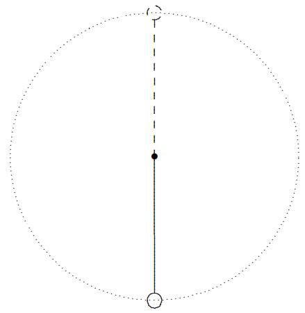
Figure \( 3.5\): A mass on a rigid rod, free to swing in the earth’s gravity in a vertical plane.

When the mass is at the unstable equilibrium point, the smallest disturbance will cause it to fall. Once away from equilibrium, the displacement increases exponentially until the angle from the vertical becomes so large that the nonlinearities in the equation of motion for this system take over. We will discuss this nonlinear oscillator further in appendix B.

Once we have found the possible values of \(\omega^{2}\), we can put each one back into (3.72) to get the corresponding \(A\). Because (3.72) is homogeneous, the overall scale of \(A\) is not determined, but all the ratios, \(a_{j} / a_{k}\), are fixed for each \(\omega^{2}\).

Normal Modes and Frequencies

The vector \(A\) is called the “normal mode” of the system associated with the frequency \(\omega\). Because \(A\) is real, in the absence of friction, the complex solutions, (3.66), can be put together into real solutions, like (3.69). The general real solution is of the form \[\begin{gathered}
X(t)=\operatorname{Re}[(b+i c) Z(t)]= \\
b A \cos \omega t+c A \sin \omega t=d A \cos (\omega t-\theta)
\end{gathered}\]

where \(b\) and \(c\) (or \(d\) and \(\theta\)) are real numbers.

We can now construct the complete solution to the equation of motion. Because of linearity, we get it by adding together all the normal mode solutions with arbitrary coefficients that must be set by the initial conditions.

We can now see that the number of different normal modes is always equal to \(n\), the number of degrees of freedom. Label the normal modes as \(A^{\alpha}\), where \(\alpha\) is a label that (we will argue below) goes from 1 to \(n\). Label the corresponding frequencies \(\omega_{\alpha}\). Then the most general possible motion of the system is a sum of all the normal modes, \[Z(t)=\sum_{\alpha=1}^{n} w_{\alpha} A^{\alpha} e^{-i \omega_{\alpha} t}\]

or in real form (with \(w = b + ic\)) \[\begin{aligned}
X(t)=& \sum_{\alpha=1}^{n}\left[b_{\alpha} A^{\alpha} \cos \left(\omega_{\alpha} t\right)+c_{\alpha} A^{\alpha} \sin \left(\omega_{\alpha} t\right)\right] \\
&=\sum_{\alpha=1}^{n} d_{\alpha} A^{\alpha} \cos \left(\omega_{\alpha} t-\theta_{\alpha}\right)
\end{aligned}\]

where \(b_{\alpha}\) and \(c_{\alpha}\) (or \(d_{\alpha}\) and \(\theta_{\alpha}\)) are real numbers that must be determined from the initial conditions of the system. Note that the set of all the normal mode vectors must be “complete,” in the mathematical sense that any possible configuration of this system can be described as a linear combination of normal modes. Otherwise, we could not satisfy arbitrary initial conditions with the solution, (3.76). This can be proved mathematically (because the matrix, \(K\), is symmetric and the masses are positive), but the physical argument will be enough for us here. Likewise no normal mode can possibly be a linear combination of the other normal modes, because each corresponds to an independent possible motion of the physical system with its own frequency. The mathematical way of saying this is that the set of all the normal modes is “linearly independent.”

Because the set of normal modes must be both complete and linearly independent, there must be precisely \(n\) normal modes, where again, \(n\) is the (3.77) number of degrees of freedom.

If there were fewer than \(n\) normal modes, they could not possibly describe all possible configurations of the \(n\) degrees of freedom. If there were more than \(n\), they could not be linearly independent \(n\) dimensional vectors. At least one of them could be written as a linear combination of the others. As we will see later, (3.77) is the physical principle behind Fourier analysis.

It is worth noting that solving the eigenvalue equation, (3.68), gets hard very rapidly as the number of degrees of freedom increases. First you have to compute the determinant of an \(n \times n\) matrix. If all the entries are nonzero, this requires adding up \(n!\) terms. Once you have finished that, you still have to solve a polynomial equation of degree \(n\). For \(n > 3\), this cannot be done analytically except in special cases.

On the other hand, it is always straightforward to check whether a given vector is an eigenvector of a given matrix and, if so, to compute the eigenvalue. We will use this fact in the problems at the end of the chapter.

Back to the \(2 \times 2\) Example

Let us return to the example from the beginning of this chapter in the special case where the two pendulum blocks have the same mass, \(m_{1} = m_{2} = m\). Simple as it is, this will be a very important system for our understanding of wave phenomena. Let us see how the techniques that we have developed allow us to solve for the allowed frequencies and the corresponding \(A\) vectors, the normal modes. From (3.7) and (3.8), the \(K\) matrix has the form \[K=\left(\begin{array}{cc}
m g / \ell+\kappa & -\kappa \\
-\kappa & m g / \ell+\kappa
\end{array}\right) .\]

The \(M\) matrix is \[M=\left(\begin{array}{cc}
m & 0 \\
0 & m
\end{array}\right) .\]

Thus from (3.78) and (3.79), \[M^{-1} K=\left(\begin{array}{cc}
g / \ell+\kappa / m & -\kappa / m \\
-\kappa / m & g / \ell+\kappa / m
\end{array}\right) .\]

The matrix \(M^{-1}K − \omega^{2}I\) is \[M^{-1} K-\omega^{2} I=\left(\begin{array}{cc}
g / \ell+\kappa / m-\omega^{2} & -\kappa / m \\
-\kappa / m & g / \ell+\kappa / m-\omega^{2}
\end{array}\right) .\]

To find the eigenvalues of \(M^{-1}K\), we form the determinant \[\begin{gathered}
\operatorname{det}\left[M^{-1} K-\omega^{2} I\right]=\operatorname{det}\left[\left(\begin{array}{cc}
g / \ell+\kappa / m-\omega^{2} & -\kappa / m \\
-\kappa / m & g / \ell+\kappa / m-\omega^{2}
\end{array}\right)\right] \\
=\left(g / \ell+\kappa / m-\omega^{2}\right)^{2}-(\kappa / m)^{2} \\
=\left(\omega^{2}-g / \ell\right)\left(\omega^{2}-g / \ell-2 \kappa / m\right)=0 .
\end{gathered}\]

Thus the angular frequencies of the normal modes are \[\omega_{1}^{2}=g / \ell, \quad \omega_{2}^{2}=g / \ell+2 \kappa / m .\]

To find the corresponding normal modes, we substitute these frequencies back into the eigenvalue equation. For \(\omega_{1}^{2}\), the normal mode vector, \(A^{1}\), \[A^{1}=\left(\begin{array}{l}
a_{1}^{1} \\
a_{2}^{1}
\end{array}\right) ,\]

satisfies the matrix equation \[\left[M^{-1} K-\omega_{1}^{2} I\right] A^{1}=0 .\]

From (3.81) and (3.83), \[M^{-1} K-\omega_{1}^{2} I=\left(\begin{array}{cc}
\kappa / m & -\kappa / m \\
-\kappa / m & \kappa / m
\end{array}\right) .\]

Thus (3.85) becomes \[\begin{aligned}
&\left(\begin{array}{cc}
\kappa / m & -\kappa / m \\
-\kappa / m & \kappa / m
\end{array}\right)\left(\begin{array}{l}
a_{1}^{1} \\
a_{2}^{1}
\end{array}\right)=0 \\
&=\frac{\kappa}{m}\left(\begin{array}{c}
a_{1}^{1}-a_{2}^{1} \\
-a_{1}^{1}+a_{2}^{1}
\end{array}\right) \Rightarrow a_{1}^{1}=a_{2}^{1} .
\end{aligned}\]

We can take \(a_{1}^{1}=1\) because we can multiply the normal mode vector by any number we like. Only the ratio \(a_{1}^{1} / a_{2}^{1}\) matters. So, for example, we can take \[A^{1}=\left(\begin{array}{l}
1 \\
1
\end{array}\right) .\]

This gives (3.10). The displacement in this normal mode is shown in Figure \( 3.6\).

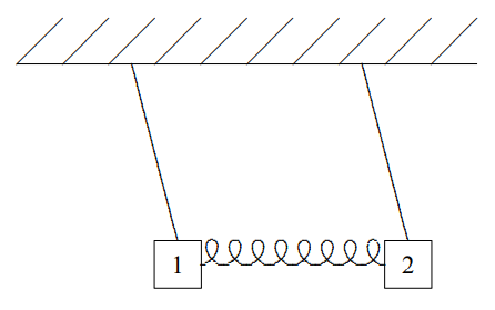
Figure \( 3.6\): The displacement in the normal mode, \(A^{1}\).

For \(\omega_{2}^{2}\), the normal mode vector, \(A^{2}\), \[A^{2}=\left(\begin{array}{l}
a_{1}^{2} \\
a_{2}^{2}
\end{array}\right) ,\]

satisfies the matrix equation (where the identity matrix multiplying \(\omega_{2}^{2}\) is understood)³ \[\left[M^{-1} K-\omega_{2}^{2}\right] A^{2}=0 .\]

This time, (3.81) and (3.83) give \[M^{-1} K-\omega_{2}^{2}=\left(\begin{array}{cc}
-\kappa / m & -\kappa / m \\
-\kappa / m & -\kappa / m
\end{array}\right) .\]

Thus (3.90) becomes \[\begin{aligned}
&\left(\begin{array}{ll}
-\kappa / m & -\kappa / m \\
-\kappa / m & -\kappa / m
\end{array}\right)\left(\begin{array}{l}
a_{1}^{2} \\
a_{2}^{2}
\end{array}\right)=0 \\
&=-\frac{\kappa}{m}\left(\begin{array}{l}
a_{1}^{2}+a_{2}^{2} \\
a_{1}^{2}+a_{2}^{2}
\end{array}\right) \Rightarrow a_{1}^{2}=-a_{2}^{2} .
\end{aligned} .\]

Again, only the ratio \(a_{1}^{2} / a_{2}^{2}\) matters, so we can take \[A^{2}=\left(\begin{array}{c}
1 \\
-1
\end{array}\right) .\]

This gives (3.11). The displacement in this normal mode is shown in Figure \( 3.7\).

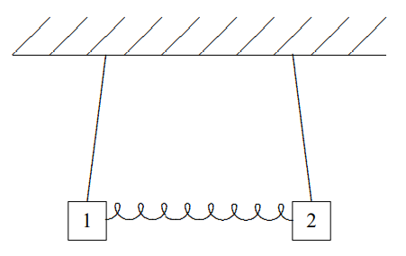
Figure \( 3.7\): The displacement in the normal mode, \(A^{2}\).

The physics of these modes is easy to understand. In mode 1, the blocks move together and the spring is never stretched from its equilibrium position. Thus the frequency is just \(g / \ell\), the same as an uncoupled pendulum. In mode 2, the blocks are moving in opposite directions, so the spring is stretched by twice the displacement of each block. Thus there is an additional restoring force of \(2\kappa\), and the square of the angular frequency is correspondingly larger.

\(n=2\) — the General Case

Let us work out explicitly the case of \(n = 2\) for an arbitrary \(K\) matrix, \[M^{-1} K=\left(\begin{array}{ll}
K_{11} / m_{1} & K_{12} / m_{1} \\
K_{12} / m_{2} & K_{22} / m_{2}
\end{array}\right) ,\]

where we have used \(K_{21} = K_{12}\). Then (3.73) becomes \[\left(\frac{K_{11} K_{22}-K_{12}^{2}}{m_{1} m_{2}}\right)-\left(\frac{K_{11}}{m_{1}}+\frac{K_{22}}{m_{2}}\right) \omega^{2}+\omega^{4}=0 ,\]

with solutions \[\omega^{2}=\frac{1}{2}\left(\frac{K_{11}}{m_{1}}+\frac{K_{22}}{m_{2}}\right) \pm \sqrt{\frac{1}{4}\left(\frac{K_{11}}{m_{1}}-\frac{K_{22}}{m_{2}}\right)^{2}+\frac{K_{12}^{2}}{m_{1} m_{2}}} .\]

For each \(\omega^{2}\), we can take \(a_{1} = 1\). Then \[a_{2}=\frac{m_{1} \omega^{2}-K_{11}}{K_{12}} .\]

As we anticipated, the eigenvectors turned out to be real. This a general consequence of the reality of \(M^{-1}K\) and \(\omega^{2}\). The argument is worth repeating. When all the elements of the matrix \(M^{-1}K − \omega^{2}I\) are real, the ratios, \(a_{j} / a_{k}\) are real (because they are obtained by solving a set of simultaneous linear equations with real coefficients). Thus if we choose one component of the vector \(A\) to be real (multiplying, if necessary, by a complex number), then all the components will be real. Physically, this means that for the solution, (3.66), all the different parts of the system are oscillating not only with the same frequency, but with the same phase up to a sign. This is true only because we have ignored damping. We will return to the question in the last section (an optional section that is not for the fainthearted).

Initial Value Problem

Once you have solved for the normal modes and corresponding frequencies, it is straightforward to put them together into the most general solution to the equations of motion for the set of \(N\) coupled oscillators, (3.76). It is \[X(t)=\sum_{\alpha}\left(b_{\alpha} A^{\alpha} \cos \omega_{\alpha} t+c_{\alpha} A^{\alpha} \sin \omega_{\alpha} t\right) .\]

The \(2N\) constants \(b_{\alpha}\) and \(c_{\alpha}\) are determined by the initial conditions. The \(b_{\alpha}\) are related to the initial displacements, \(X(0)\): \[X(0)=\sum_{\alpha} b_{\alpha} A^{\alpha} .\]

In words, \(b_{\alpha}\) is the coefficient of the normal mode \(A^{\alpha}\) in the initial displacement \(X(0)\). The \(c_{\alpha}\) are related to the initial velocities, \(\left.\frac{d X(t)}{d t}\right|_{t=0}\): \[\left.\frac{d X(t)}{d t}\right|_{t=0}=\sum_{\alpha} c_{\alpha} \omega_{\alpha} A^{\alpha} .\]

The equations, (3.99) and (3.100), are two sets of simultaneous linear equations for the \(b_{\alpha}\) and \(c_{\alpha}\). They can be solved by hand. This is easy enough for a small number of degrees of freedom. We will see in the next section that we can also get the solutions directly with very little additional work by manipulating the normal modes.

Meanwhile, we should pause again to consider the physics of (3.98). This shows explicitly how the most general motion of the system can be decomposed into the simple motions associated with the normal modes. It is worth staring at an example (real, animated or preferably both) at this point. Try to construct the system in Figure \( 3.1\). Any two identical oscillators with a relatively weak spring connecting them will do. Convince yourself that the normal modes exist. If you start the system oscillating with the blocks moving the same way with the same amplitude, they will stay that way. If you get them started moving in opposite directions with the same amplitude, they will continue doing that. Now set up a random motion. See if you can understand how to take it apart into normal modes. It may help to stare again at program 3-1 on the program disk, in which this is done explicitly. In this animation, you see the two blocks of Figure \( 3.1\) and below, the two normal modes that must be added to produce the full solution.

_______________________
³It is tiresome writing the identity matrix, \(I\), everywhere. It is not really necessary because you can always tell from the context whether it belongs there or not. From now on, we will often leave it out. Thus, if you see something that looks like a number in a matrix equation, like the \(-\omega_{2}^{2}\) in (3.90), you should mentally include a factor of \(I\).