Physics LibreTexts

3.5: * Forced Oscillations and Resonance

  • Page ID
    34362
  • \( \newcommand{\vecs}[1]{\overset { \scriptstyle \rightharpoonup} {\mathbf{#1}} } \) \( \newcommand{\vecd}[1]{\overset{-\!-\!\rightharpoonup}{\vphantom{a}\smash {#1}}} \)\(\newcommand{\id}{\mathrm{id}}\) \( \newcommand{\Span}{\mathrm{span}}\) \( \newcommand{\kernel}{\mathrm{null}\,}\) \( \newcommand{\range}{\mathrm{range}\,}\) \( \newcommand{\RealPart}{\mathrm{Re}}\) \( \newcommand{\ImaginaryPart}{\mathrm{Im}}\) \( \newcommand{\Argument}{\mathrm{Arg}}\) \( \newcommand{\norm}[1]{\| #1 \|}\) \( \newcommand{\inner}[2]{\langle #1, #2 \rangle}\) \( \newcommand{\Span}{\mathrm{span}}\) \(\newcommand{\id}{\mathrm{id}}\) \( \newcommand{\Span}{\mathrm{span}}\) \( \newcommand{\kernel}{\mathrm{null}\,}\) \( \newcommand{\range}{\mathrm{range}\,}\) \( \newcommand{\RealPart}{\mathrm{Re}}\) \( \newcommand{\ImaginaryPart}{\mathrm{Im}}\) \( \newcommand{\Argument}{\mathrm{Arg}}\) \( \newcommand{\norm}[1]{\| #1 \|}\) \( \newcommand{\inner}[2]{\langle #1, #2 \rangle}\) \( \newcommand{\Span}{\mathrm{span}}\)\(\newcommand{\AA}{\unicode[.8,0]{x212B}}\)

    One of the advantages of the matrix formalism that we have introduced is that in matrix language we can take over the above discussion of forced oscillation and resonance in chapter 2 almost unchanged to systems with more than one degree of freedom. We simply have to replace numbers by appropriate vectors and matrices. In particular, the force \(F(t)\) in the equation of motion, (2.2), becomes a vector that describes the force on each of the degrees of freedom in the system. The only restriction here is that the frequency of oscillation is the same for each component of the force. The \(\omega_{0}^{2}\) in the equation of motion, (2.2), becomes the matrix \(M^{-1}K\). The frictional term \(\Gamma\) becomes a matrix. In terms of the matrix \(\Gamma\), the frictional force vector is \(M \Gamma d Z / d t\) (compare (2.1)). Then we can look for an irreducible, steady state solution to the equation of motion of the form \[Z(t)=W e^{-i \omega t}\]

    where \(W\) is a constant vector, which yields the matrix equation \[\left[-\omega^{2}-i \Gamma \omega+M^{-1} K\right\rceil W=M^{-1} F_{0} .\]

    Formally, we can solve this by multiplying by the inverse matrix \[W=\left[M^{-1} K-\omega^{2}-i \Gamma \omega\right]^{-1} M^{-1} F_{0} .\]

    If \(\Gamma\) were zero in the matrix \[\left[-\omega^{2}-i \Gamma \omega+M^{-1} K\right] ,\]

    then we know that the inverse matrix would not exist for any value of \(\omega\) corresponding to a free oscillation frequency of the system, \(\omega_{0}\), because the determinant of the \(M^{-1} K-\omega_{0}^{2}\) matrix is zero. The amplitude \(W\) would go to \(\infty\) in this limit, in the direction of the normal mode associated with the driving frequency, so long as the driving force has a component in the normal mode direction. For \(\omega\) close to \(\omega_{0}\), if there is no damping, the response amplitude is very large, proportional to \(1 /\left(\omega_{0}^{2}-\omega^{2}\right)\), almost in the direction of the normal mode. However, in the presence of damping, the response amplitude does not go to \(\infty\) even for \(\omega = \omega_{0}\), because the \(i \Gamma \omega\) term is still nonvanishing.

    We can see all this explicitly if the damping matrix \(\Gamma\) is proportional to the identity matrix, \[\Gamma=\gamma I .\]

    Then we can use (3.124)-(3.126) to write \(\left[M^{-1} K-\omega^{2}-i \Gamma \omega\right]\) as a sum over the normal modes, as follows: \[\left[M^{-1} K-\omega^{2}-i \Gamma \omega\right]=\sum_{\alpha}\left(\omega_{\alpha}^{2}-\omega^{2}-i \gamma \omega\right) \frac{A^{\alpha} B^{\alpha}}{B^{\alpha} A^{\alpha}} .\]

    Then the inverse matrix can be constructed in a similar way, just by inverting the factor in the numerator: \[\left[M^{-1} K-\omega^{2}-i \Gamma \omega\right]^{-1}=\sum_{\alpha}\left(\omega_{\alpha}^{2}-\omega^{2}-i \gamma \omega\right)^{-1} \frac{A^{\alpha} B^{\alpha}}{B^{\alpha} A^{\alpha}} .\]

    Using (3.137), we can rewrite (3.133) as \[W=\sum_{\alpha} \frac{\Lambda^{\alpha}}{\omega_{\alpha}^{2}-\omega^{2}-i \gamma \omega} \frac{B^{\alpha} M^{-1} F_{0}}{B^{\alpha} A^{\alpha}} .\]

    This has a simple interpretation. The second factor on the right hand side of (3.138) is the coefficient of the normal mode \(A^{\alpha}\) in the driving term, \(M^{-1} F_{0}\). This coefficient is multiplied by the complex number \[\left[\frac{1}{\omega_{\alpha}^{2}-\omega^{2}-i \gamma \omega}\right] ,\]

    which is exactly analogous to the factor in (2.21) in the one dimensional case. Thus if \(\Gamma \propto I\), then, for each normal mode, the forced oscillation works just as it does for one degree of freedom. If \(\Gamma\) is not proportional to the identity matrix, the formulas are a bit more complicated, but the physics is qualitatively the same.

    Example

    We will illustrate these considerations with our favorite example, the system of two identical coupled oscillators, with \(M^{-1}K\) matrix given by (3.80). We will imagine that the system is sitting in a viscous fluid that gives a uniform damping \(\Gamma = \gamma I\), and that there is a periodic force that acts twice as strongly on block 1 as on block 2 (for example, we might give the blocks electric charge \(2q\) and \(q\) and subject them to a periodic electric field), so that the force is \[F(t)=\left(\begin{array}{l}
    2 \\
    1
    \end{array}\right) f_{0} \cos \omega t=\operatorname{Re}\left[\left(\begin{array}{l}
    2 \\
    1
    \end{array}\right) f_{0} e^{-i \omega t}\right] .\]

    Thus \[M^{-1} F_{0}=\left(\begin{array}{l}
    2 \\
    1
    \end{array}\right) \frac{f_{0}}{m} .\]

    Now to use (3.133), we need only invert the matrix \[\left[M^{-1} K-\omega^{2}-i \Gamma \omega\right]=\left(\begin{array}{cc}
    \frac{g}{\ell}+\frac{\kappa}{m}-\omega^{2}-i \gamma \omega & -\frac{\kappa}{m} \\
    -\frac{\kappa}{m} & \frac{g}{\ell}+\frac{\kappa}{m}-\omega^{2}-i \gamma \omega
    \end{array}\right) .\]

    This is simple enough to do by hand. We will do that first, and then compare the result with (3.137). The determinant is \[\begin{gathered}
    \left(\frac{g}{\ell}+\frac{\kappa}{m}-\omega^{2}-i \gamma \omega\right)^{2}-\left(\frac{\kappa}{m}\right)^{2} \\
    =\left(\frac{g}{\ell}+2 \frac{\kappa}{m}-\omega^{2}-i \gamma \omega\right) \cdot\left(\frac{g}{\ell}-\omega^{2}-i \gamma \omega\right) .
    \end{gathered}

    Applying (3.34), we find \[\begin{gathered}
    {\left[M^{-1} K-\omega^{2}-i \Gamma \omega\right]^{-1}} \\
    =\frac{1}{\left(\frac{g}{\ell}+2 \frac{\kappa}{m}-\omega^{2}-i \gamma \omega\right)\left(\frac{g}{\ell}-\omega^{2}-i \gamma \omega\right)} \\
    \cdot\left(\begin{array}{cc}
    \frac{g}{\ell}+\frac{\kappa}{m}-\omega^{2}-i \gamma \omega & \frac{\kappa}{m} \\
    \frac{\kappa}{m} & \frac{g}{\ell}+\frac{\kappa}{m}-\omega^{2}-i \gamma \omega
    \end{array}\right) .
    \end{gathered}\]

    If we isolate the contribution of the two zeros in the denominator of (3.144), we can write \[\begin{gathered}
    {\left[M^{-1} K-\omega^{2}-i \Gamma \omega\right]^{-1}} \\
    =\frac{1}{2} \frac{1}{\left(\frac{g}{\ell}-\omega^{2}-i \gamma \omega\right)}\left(\begin{array}{ll}
    1 & 1 \\
    1 & 1
    \end{array}\right) \\
    +\frac{1}{2} \frac{1}{\left(\frac{g}{\ell}+2 \frac{\kappa}{m}-\omega^{2}-i \gamma \omega\right)}\left(\begin{array}{cc}
    1 & -1 \\
    -1 & 1
    \end{array}\right)
    \end{gathered}\)

    which is just (3.137), as promised. Now substituting into (3.133), we find \[\begin{gathered}
    W=\frac{1}{2} \frac{1}{\left(\frac{g}{\ell}-\omega^{2}-i \gamma \omega\right)}\left(\begin{array}{l}
    3 \\
    3
    \end{array}\right) \frac{f_{0}}{m} \\
    +\frac{1}{2} \frac{1}{\left(\frac{g}{\ell}+2 \frac{\kappa}{m}-\omega^{2}-i \gamma \omega\right)}\left(\begin{array}{c}
    1 \\
    -1
    \end{array}\right) \frac{f_{0}}{m} \\
    =\frac{1}{2} \frac{\left(\frac{g}{\ell}-\omega^{2}+i \gamma \omega\right)}{\left(\frac{g}{\ell}-\omega^{2}\right)^{2}+(\gamma \omega)^{2}}\left(\begin{array}{l}
    3 \\
    3
    \end{array}\right) \frac{f_{0}}{m} \\
    +\frac{1}{2} \frac{\left(\frac{g}{\ell}+2 \frac{\kappa}{m}-\omega^{2}+i \gamma \omega\right)}{\left(\frac{g}{\ell}+2 \frac{\kappa}{m}-\omega^{2}\right)^{2}+(\gamma \omega)^{2}}\left(\begin{array}{c}
    1 \\
    -1
    \end{array}\right) \frac{f_{0}}{m},
    \end{gathered}\]

    from which we can read off the final result: \[X(t)=\operatorname{Re}\left(W e^{-i \omega t}\right)=\left(\begin{array}{l}
    \alpha_{1} \cos \omega t+\beta_{1} \sin \omega t \\
    \alpha_{2} \cos \omega t+\beta_{2} \sin \omega t
    \end{array}\right)\]

    where \[\begin{aligned}
    &\alpha_{1(2)}=\frac{3}{2} \frac{\left(\frac{g}{\ell}-\omega^{2}\right)}{\left(\frac{g}{\ell}-\omega^{2}\right)^{2}+(\gamma \omega)^{2}} \frac{f_{0}}{m} \\
    &\pm \frac{1}{2} \frac{\left(\frac{g}{\ell}+2 \frac{\kappa}{m}-\omega^{2}\right)}{\left(\frac{g}{\ell}+2 \frac{\kappa}{m}-\omega^{2}\right)^{2}+(\gamma \omega)^{2}} \frac{f_{0}}{m}
    \end{aligned}\]

    and \[\begin{aligned}
    &\beta_{1(2)}=\frac{3}{2} \frac{\gamma \omega}{\left(\frac{g}{\ell}-\omega^{2}\right)^{2}+(\gamma \omega)^{2}} \frac{f_{0}}{m} \\
    &\pm \frac{1}{2} \frac{\gamma \omega}{\left(\frac{g}{\ell}+2 \frac{\kappa}{m}-\omega^{2}\right)^{2}+(\gamma \omega)^{2}} \frac{f_{0}}{m} .
    \end{aligned}\]

    The power expended by the external force is the sum over all the degrees of freedom of the force times the velocity. In matrix language, this can be written as \[P(t)=F(t)^{T} \cdot \frac{d X(t)}{d t} .\]

    The average power lost to the frictional force comes from the \(\cos ^{2} \omega t\) term in (3.150) and is \[\begin{aligned}
    &=\frac{1}{\left(\frac{g}{\ell}-\omega^{2}\right)^{2}+(\gamma \omega)^{2}} \frac{9 \gamma \omega^{2} f_{0}^{2}}{4 m} \\
    &+\frac{1}{\left(\frac{g}{\ell}+2 \frac{\kappa}{m}-\omega^{2}\right)^{2}+(\gamma \omega)^{2}} \frac{\gamma \omega^{2} f_{0}^{2}}{4 m}
    \end{aligned}\]

    Figure \( 3.8\) shows a graph of this (for \(\kappa / m=3 g / 2 \ell\) and \(\gamma^{2}=g / 4 \ell\)). There are two things to observe about Figure \( 3.8\). First note the two resonance peaks, at \(\omega^{2} = g / \ell\) and \(\omega^{2}=g / \ell+2 \kappa / m=4 g / \ell\). Secondly, note that the first peak is much more pronounced that the second. That is because the force is more in the direction of the normal mode with the lower frequency, thus it is more efficient in exciting this mode.
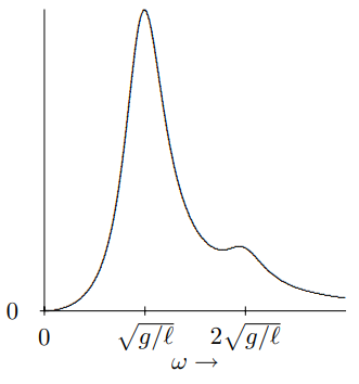
    clipboard_e76fa192ca328062f106e953071352727.png

    Figure \( 3.8\): The average power lost to friction in the example of 3.140.


    This page titled 3.5: * Forced Oscillations and Resonance is shared under a CC BY-NC-SA 4.0 license and was authored, remixed, and/or curated by Howard Georgi via source content that was edited to the style and standards of the LibreTexts platform; a detailed edit history is available upon request.