10.4: Scattering of Wave Packets

In a real scattering experiment, we are interested not in an incoming harmonic wave that has always existed and will always exist. Instead we are interested in an incoming wave packet that is limited in time. In this section, we discuss two examples of scattering of wave packets.

Scattering from a Boundary

10-3
We begin with the easier of the two examples. Consider the scattering of a wave packet from the boundary between two semi-infinite dispersionless strings both with tension \(T\) and different densities, \(\rho_{I}\) and \(\rho_{II}\), as shown in Figure \( 9.1\). The dispersion relations are: \[\omega^{2}=\left\{\begin{array}{l}
v_{I}^{2} k^{2}=\frac{T}{\rho_{I}} k^{2}=\quad \text { in region } I \\
v_{I I}^{2} k^{2}=\frac{T}{\rho_{I I}} k^{2} \quad \text { in region } I I
\end{array}\right.\]

where \(v_{I}\) and \(v_{II}\) are the phase velocities in the two regions.

Specifically, we assume that the boundary condition at \(-\infty\) is that there is an incoming wave, \[f(x-v t)\]

in region \(I\), but no incoming wave in region \(II\), and we wish to find the outgoing waves, the reflected wave in region \(I\) and the transmitted wave in region \(II\).

We can solve this problem without decomposing the wave packet into its harmonic components with a trick that is analogous to that used at the beginning of this chapter to solve the forced oscillation problem, Figure \( 10.1\). The most general solution to the boundary conditions at \(\pm \infty\) is \[\psi(x, t)= \begin{cases}f\left(t-x / v_{I}\right)+g\left(t+x / v_{I}\right) & \text { in region } I \\ h\left(t-x / v_{I I}\right) & \text { in region } I I\end{cases}\]

where \(g\) and \(h\) are arbitrary functions. To actually determine the reflected and transmitted waves, we must impose the boundary conditions at \(x = 0\), that the displacement is continuous (because the string doesn’t break) and its x derivative is continuous (because the knot joining the two strings is massless): \[f(t)+g(t)=h(t) ,\]

and \[\left.\frac{\partial}{\partial x}\left[f\left(t-x / v_{I}\right)+g\left(t+x / v_{I}\right)\right]\right|_{x=0}=\left.\frac{\partial}{\partial x} h\left(t-x / v_{I I}\right)\right|_{x=0} .\]

Using the chain rule in (10.79), we can relate the partial derivatives with respect to \(x\) to deriviatives of the functions, \[\left.\frac{1}{v_{I}}\left[-f^{\prime}\left(t-x / v_{I}\right)+g^{\prime}\left(t+x / v_{I}\right)\right]\right|_{x=0}=-\left.\frac{1}{v_{I I}} h^{\prime}\left(t-x / v_{I I}\right)\right|_{x=0} ,\]

or \[-f^{\prime}(t)+g^{\prime}(t)=-\frac{v_{I}}{v_{I I}} h^{\prime}(t) .\]

Differentiating (10.78), we get \[f^{\prime}(t)+g^{\prime}(t)=h^{\prime}(t) ,\]

Now for every value of \(t\), (10.81) and (10.82) form a pair of simultaneous linear equations that can be solved for \(g^{\prime}(t)\) and \(h^{\prime}(t)\) in terms of \(f^{\prime}(t)\): \[g^{\prime}(t)=\frac{1-v_{I} / v_{I I}}{1+v_{I} / v_{I I}} f^{\prime}(t), \quad h^{\prime}(t)=\frac{2}{1+v_{I} / v_{I I}} f^{\prime}(t) .\]

Undoing the derivatives, we can write \[g(\iota)=\frac{1-v_{I} / v_{I I}}{1+v_{I} / v_{I I}} \int(\iota)+k_{1}, \quad h(\iota)=\frac{2}{1+v_{I} / v_{I I}} \int(\iota)+k_{2} .\]

where \(k_{1}\) and \(k_{2}\) are constants, independent of \(t\). In fact, though, we must have \(k_{1} = k_{2}\) to satisfy (10.78), and adding the same constant in both regions is irrelevant, because it just corresponds to our freedom to move the whole string up or down in the transverse direction. Thus we conclude that \[g(t)=\frac{1-v_{I} / v_{I I}}{1+v_{I} / v_{I I}} f(t), \quad h(t)=\frac{2}{1+v_{I} / v_{I I}} f(t) ,\]

and the solution, (10.77), becomes \[\psi(x, t)= \begin{cases}f\left(t-x / v_{I}\right)+\frac{1-v_{I} / v_{I I}}{1+v_{I} / v_{I I}} f\left(t+x / v_{I}\right) & \text { in region } I, \\ \frac{2}{1+v_{I} / v_{I I}} f\left(t-x / v_{I I}\right) & \text { in region } I I .\end{cases}\]

The same result emerges if we take the incoming wave packet apart into its harmonic components. For each harmonic component, the reflection and transmission components are the same (from (9.16)):

When we now put the harmonic components back together to get the scatter and transmitted wave packets, the coefficients, \(\rho\) and \(\tau\) appear just as overall constants in front of the original pulse, as in (10.86).

This scattering process is animated in program 10-3. Here you can input different values of \(v_{I I} / v_{I}\) to see how the reflection and transmission is affected. Notice that \(v_{I I} / v_{I}\) very small corresponds to a large impedance ratio, \(Z_{I I} / Z_{I}\), which means that the string in region \(II\) does not move very much. Then we get a reflected pulse that is just the incoming pulse flipped over below the string. In the extreme limit, \(v_{I I} / v_{I} \rightarrow \infty\), the boundary at \(x = 0\) acts like a fixed end. \(v_{I I} / v_{I}\) very large corresponds to a small impedance ratio, \(Z_{I I} / Z_{I}\), in which case the string in region \(I\) hardly notices the string in region \(II\). In the limit \(v_{I I} / v_{I} \rightarrow 0\), the boundary at \(x = 0\) acts like a free end.

Mass on a String

10-4
A more interesting example of the scattering of wave packets that can be worked out using the mathematics we have already done is the scattering of an incoming wave packet with the shape of (10.39) encountering a mass on a string. Here the dispersion relation is trivial, so the wave packet propagates without change of shape until it “hits” the mass. But then interesting things happen. This time, when we decompose the wave packet into its harmonic components, the reflection and transmission coefficients depend on \(\omega\). When we add them

Figure \( 10.6\): A mass on a string.

back up again to get the reflected and transmitted wave packets, we will find that the shape has changed. We will work this out in detail. The familiar setup is shown in Figure \( 10.6\).

For an incoming harmonic wave of amplitude \(A\), the displacement looks like \[\psi(x, t)=A e^{i k x} \cdot e^{-i \omega t}+R A e^{-i k x} \cdot e^{-i \omega t} \text { for } x \leq 0\]

\[\psi(x, t)=\tau A e^{i k x} \cdot e^{-i \omega t} \text { for } x \geq 0\]

The solution for \(R\) and \(\tau\) was worked out in the last chapter in (9.39)-(9.45). However, the parameter \(\epsilon\) of (9.38) depends on \(\omega\). In order to disentangle the frequency dependence of the scattered wave packets, we write \(R\) and \(\tau\) as \[\tau=\frac{2 \Omega}{2 \Omega-i \omega}, \quad R=\frac{i \omega}{2 \Omega-i \omega} ,\]

where \[\Omega \equiv \frac{T}{m v}=\frac{\sqrt{\rho T}}{m} ,\]

is independent of \(\omega\) — it depends just on the fixed parameters of the string and the mass. Note that in the notation of (9.38), \[\Omega=\frac{\omega}{\epsilon} .\]

Suppose that we have not a harmonic incoming wave, but an incoming pulse: \[\psi_{\mathrm{in}}(x-v t)=A e^{-\Gamma|t-x / v|} .\]

Now the situation is more interesting. We expect a solution of the form \[\begin{aligned}
&\begin{aligned}
&\hline
\end{aligned}\\
&8
\end{aligned}\]

\[\psi(x, t)=\psi_{\tau}(x-v t) \text { for } x \geq 0\]

where \(\psi_{\tau}(x+v t)\] is the transmitted wave, traveling in the \(+x\) direction, and \(\psi_{R}(x+v t)\) is the reflected wave, traveling in the \(-x\) direction. To get the reflected and transmitted waves, we will use superposition and take \(\psi_{in}\) apart into harmonic components. We can then use to determine the scattering of each of the components, and then can put the pieces back together to get the solution. Thus we start by Fourier transforming \(\psi_{in}\): \[\psi_{\text {in }}(x, t)=\int d \omega e^{-i \omega(t-x / v)} C_{\text {in }}(\omega) .\]

We know from our discussion of signals that \[\begin{gathered}
C_{\text {in }}(\omega)=\frac{1}{2 \pi} \int d t e^{i \omega t} \psi_{\text {in }}(0, t) \\
=\frac{1}{2 \pi} \int_{0}^{\infty} d t A e^{i \omega t} e^{-\Gamma t}+\text { h.c. }=\frac{1}{2 \pi}\left(\frac{1}{\Gamma-i \omega}+\frac{1}{\Gamma+i \omega}\right) .
\end{gathered}\]

Now to get the reflected and transmitted pulses, we multiply the components of \(\psi_{in}\) by the reflection and transmission amplitudes \(R\) and \(\tau\) for unit \(\psi_{in}\) \[C_{\tau}(\omega)=A \frac{1}{2 \pi}\left(\frac{1}{\Gamma-i \omega}+\frac{1}{\Gamma+i \omega}\right) \frac{2 \Omega}{2 \Omega-i \omega}\]

\[C_{R}(\omega)=A \frac{1}{2 \pi}\left(\frac{1}{\Gamma-i \omega}+\frac{1}{\Gamma+i \omega}\right) \frac{i \omega}{2 \Omega-i \omega}\]

Now we have to reverse the process and find the Fourier transforms of these to get the reflected and transmitted pulses. This is straightforward, because we can rewrite (10.98) and (10.99) in terms of single poles in \(\omega\): \[\begin{aligned}
C_{\tau}(\omega) &=A \frac{1}{2 \pi} \frac{2 \Omega}{2 \Omega-\Gamma} \cdot\left(\frac{1}{\Gamma-i \omega}-\frac{1}{2 \Omega-i \omega}\right) \\
+& \frac{1}{2 \pi} \frac{2 \Omega}{2 \Omega+\Gamma} \cdot\left(\frac{1}{\Gamma+i \omega}+\frac{1}{2 \Omega-i \omega}\right)
\end{aligned}\]

\[\begin{aligned}
&C_{R}(\omega)=A \frac{1}{2 \pi} \frac{1}{2 \Omega-\Gamma} \cdot\left(\frac{\Gamma}{\Gamma-i \omega}-\frac{2 \Omega}{2 \Omega-i \omega}\right) \\
&+\frac{1}{2 \pi} \frac{1}{2 \Omega+\Gamma} \cdot\left(-\frac{\Gamma}{\Gamma+i \omega}+\frac{2 \Omega}{2 \Omega-i \omega}\right) .
\end{aligned}\]

Now we can work backwards in (10.100) and (10.101) to get the Fourier transforms. We know from (10.55) that each term is the Fourier transform of an exponential. It is straight-forward, but tedious, to put them back together. The result is reproduced below (note that we have combined the two terms in each expression proportional to \(1 /(2 \Omega-i \omega)\)). \[\begin{gathered}
\psi_{\tau}(x, t)=\frac{2 \Omega}{2 \Omega-\Gamma} \theta(t-x / v) A e^{-\Gamma(t-x / v)} \\
-\frac{4 \Omega \Gamma}{4 \Omega^{2}-\Gamma^{2}} \theta(l-x / v) A e^{-2 \Omega(t-x / v)}+\frac{2 \Omega}{2 \Omega+\Gamma} \theta(-l+x / v) A e^{\Gamma(t-x / v)}
\end{gathered}\]

and \[\begin{gathered}
\psi_{r}(x, t)=\frac{2 \Gamma}{2 \Omega-\Gamma} \theta(t+x / v) A e^{-\Gamma(t+x / v)} \\
-\frac{4 \Omega \Gamma}{4 \Omega^{2}-\Gamma^{2}} \theta(t+x / v) A e^{-2 \Omega(t+x / v)}-\frac{2 \Gamma}{2 \Omega+\Gamma} \theta(-t-x / v) A e^{\Gamma(t+x / v)}
\end{gathered}\]

where \[\theta(t)=\left\{\begin{array}{l}
1 \text { for } t \geq 0 , \\
0 \text { for } t<0 .
\end{array}\right.\]

These formulas are not very transparent or informative, but we can put them into a computer and look at the result. We will plot the result in the limit \(2 \Omega \rightarrow \Gamma\). The results, (10.102) and (10.103) look singular in this limit, but actually, the limit exists and is perfectly smooth.⁴ In \(Figures \text { } 10.7 \text {-} 10.12\), we show \(\psi(x, t)\) for \(\Gamma=v=1\) in arbitrary units, for\(t\) values from \(-2\)

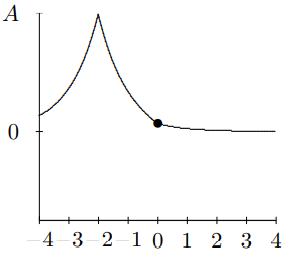
Figure \( 10.7\): A wave packet on a stretched string, at \(t = -2\).

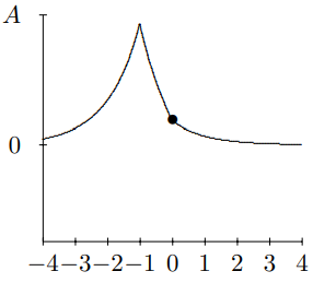
Figure \( 10.8\): \(t = -1\).

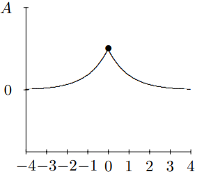
Figure \( 10.9\): \(t = 0\).

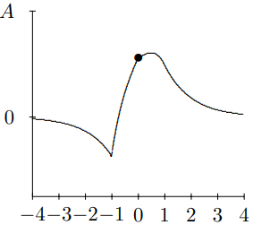
Figure \( 10.10\): \(t = 1\).

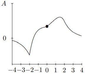
Figure \( 10.11\): \(t = 2\).

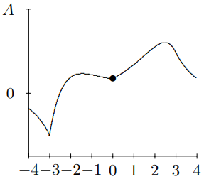
Figure \( 10.12\): \(t = 3\).

to 3. At \(t = -2\), you see the pulse approaching the mass for negative \(t\). At \(t = -1\), you can begin to see the effect of the mass on the string. By \(t = 0\), the string to the left of \(x = 0\) is moving rapidly downwards. At \(t = 1\), downward motion of the string for \(x < 0\) has continued, and has begun to form the reflected pulse. For \(t = 2\), you can see the transmitted and reflected waves beginning to separate. For \(t = 3\), you can see the reflected and transmitted pulses have separated almost completely and the mass has returned nearly to its equilibrium position. For large positive \(t\), the pulse is split into a reflected and transmitted wave.

The really interesting stuff is going on between \(t = 0\) and \(t = 1\), so we will look at this on a finer time scale in \(Figures \text { } 10.13 \text {-} 10.16\). To really appreciate this, you should see it in motion. It is animated in program 10-4.

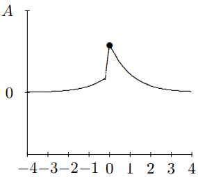
Figure \( 10.13\): This is \(t = .2\).

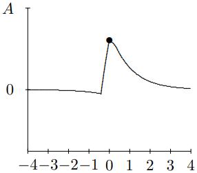
Figure \( 10.14\): This is \(t = .4\).

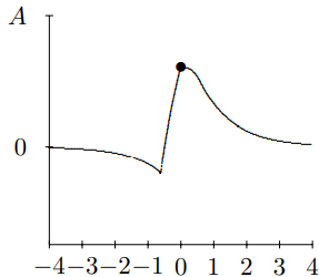
Figure \( 10.15\): This is \(t = .6\).

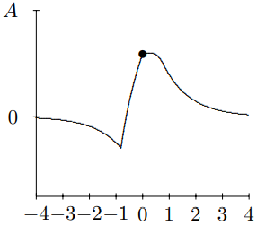
Figure \( 10.16\): This is \(t = .8\).

__________________
⁴The apparent singularity is similar to one that occurs in the approach to critical damping, discussed in (2.12).