10.3: Bandwidth, Fidelity, and Uncertainty

The relation (10.9) can be inverted to give \(C(\omega)\) in terms of \(f(t)\) as follows \[C(\omega)=\frac{1}{2 \pi} \int_{-\infty}^{\infty} d t f(t) e^{i \omega t} .\]

This is the “inverse Fourier transform.” It is very important because it allows us to go back and forth between the signal and the distribution of frequencies that it contains. We will get this result in two ways: first, with a fancy argument that we will use again and explain in more detail in chapter 13; next, by going back to the Fourier series, discussed in chapter 6 for waves on a finite string, and taking the limit as the length of the string goes to infinity.

The fancy argument goes like this. It is very reasonable that the integral in (10.37) is proportional to \(C(\omega)\) because if we insert (10.9) and rearrange the order of integration, we get \[\frac{1}{2 \pi} \int_{-\infty}^{\infty} d \omega^{\prime} C\left(\omega^{\prime}\right) \int_{-\infty}^{\infty} d t e^{i\left(\omega-\omega^{\prime}\right) t} .\]

The \(t\) integral averages to zero unless \(\omega = \omega^{\prime}\). Thus the \(\omega^{\prime}\) integral is simply proportional to \(C(\omega)\) times a constant factor. The factor of \(1 / 2 \pi\) can be obtained by doing some integrals explicitly. For example, if \[f(t)=e^{-\Gamma|t|} ,\]

for \(\Gamma>0\) then, as we will show explicitly in (10.49)-(10.56), (10.37) yields \[2 \pi C(\omega)=2 \Gamma /\left(\Gamma^{2}+\omega^{2}\right) ,\]

which can, in turn, be put back in (10.9) to give (10.39). For \(t = 0\), the integral can be done by the trigonometric substitution \(\omega \rightarrow \Gamma \tan \theta\): \[\begin{aligned}
&1=f(0)=e^{-\Gamma \cdot 0}=\int_{-\infty}^{\infty} d \omega C(\omega) e^{-i \omega \cdot 0} \\
&=\frac{1}{\pi} \int_{-\infty}^{\infty} d \omega \frac{\Gamma}{\Gamma^{2}+\omega^{2}} \rightarrow \frac{1}{\pi} \int_{-\pi / 2}^{\pi / 2} d \theta=1 .
\end{aligned}\]

To get the inverse Fourier transform, (10.37), as the limit of a Fourier series, it is convenient to use a slightly different boundary condition from those we discussed in chapter 6, fixed ends and free ends. Instead, let us consider a string stretched from \(x=-\pi \ell\) to \(x=\pi \ell\), in which we assume that the displacement of the string from equilibrium at \(x=\pi \ell\) is the same as the displacement at \(x=-\pi \ell\),² \[\psi(-\pi \ell, t)=\psi(\pi \ell, t) .\]

The requirement, (10.42), is called “periodic boundary conditions,” because it implies that the function \(\psi\) that describes the displacement of the string is periodic in \(x\) with period \(2 \pi \ell\). The normal modes of the infinite system that satisfy (10.42) are \[e^{i n x / \ell} ,\]

for integer \(n\), because changing \(x\) by \(2 \pi \ell\) in (10.43) just changes the phase of the exponential by \(2 \pi\). Thus if \(\psi(x)\) is an arbitrary function satisfying \(\psi(-\pi \ell)=\psi(\pi \ell)\), we should be able to expand it in the normal modes of (10.43), \[\psi(x)=\sum_{n=-\infty}^{\infty} c_{n} e^{-i n x / \ell} .\]

Likewise, for a function \(f(t)\), satisfying \(f(-\pi T)=f(\pi T)\) for some large time \(T\), we expect to be able to expand it as follows \[f(t)=\sum_{n=-\infty}^{\infty} c_{n} e^{-i n t / T} ,\]

where we have changed the sign in the exponential to agree with (10.9). We will show that as \(T \rightarrow \infty\), this becomes equivalent to (10.9).

Equation (10.44) is the analog of (6.8) for the boundary condition, (10.42). The sum runs from \(-\infty\) to \(\infty\) rather than 0 to \(\infty\) because the modes in (10.43) are different for \(n\) and \(-n\). For this Fourier series, the inverse is \[c_{m}=\frac{1}{2 \pi T} \int_{-\pi T}^{\pi T} d t e^{i m t / T} f(t)\]

where we have used the identity \[\frac{1}{2 \pi T} \int_{-\pi T}^{\pi T} d t e^{i m t / T} e^{-i n t / T}=\left\{\begin{array}{l}
1 \text { for } m=n , \\
0 \text { for } m \neq n .
\end{array}\right.\]

Now suppose that \(f(t)\) goes to 0 for large \(|t|\) (note that this is consistent with the periodic boundary condition (10.42)) fast enough so that the integral in (10.46) is well defined as \(T \rightarrow \infty\) for all \(m\). Then because of the factor of \(1/T\) in (10.47), the \(c_{n}\) all go to zero like \(1/T\). Thus we should multiply \(c_{n}\) by \(T\) to get something finite in the limit. Comparing (10.45) with (10.9), we see that we should take \(\omega\) to be \(n/T\).

Thus the relation, (10.45), is an analog of the Fourier integral, (10.9) where the correspondence is \[\begin{aligned}
T & \rightarrow \infty \\
\frac{n}{T} & \rightarrow \omega \\
c_{n} T & \rightarrow C(\omega) .
\end{aligned}\]

In the limit, \(T \rightarrow \infty\), the sum becomes an integral over \(\omega\).

Multiplying both sides of (10.46) by \(T\), and making the substitution of (10.48) gives (10.37).

Solvable Example

For practice in dealing with integration of complex functions, we will do the integration that leads to (10.40) in gory detail, with all the steps. \[C(\omega)=\frac{1}{2 \pi} \int_{-\infty}^{\infty} d t e^{-\Gamma|t|} e^{i \omega t} .\]

First we get rid of the absolute value — \[=\frac{1}{2 \pi} \int_{0}^{\infty} d t e^{-\Gamma t} e^{i \omega t}+\frac{1}{2 \pi} \int_{-\infty}^{0} d t e^{\Gamma t} e^{i \omega t}\]

and write the second integral as an integral from 0 to \(\infty\) — \[=\frac{1}{2 \pi} \int_{0}^{\infty} d t e^{-\Gamma t} e^{i \omega t}+\frac{1}{2 \pi} \int_{0}^{\infty} d t e^{-\Gamma t} e^{-i \omega t}\]

\[=\frac{1}{2 \pi} \int_{0}^{\infty} d t e^{-\Gamma t} e^{i \omega t}+\text { complex conjugate, }\]

but we know how to differentiate even complex exponentials (see the discussion of (3.108)), so we can write \[\frac{\partial}{\partial t}\left(e^{-\Gamma t} e^{i \omega t}\right)=(-\Gamma+i \omega) e^{-\Gamma t} e^{i \omega t} .\]

Thus \[\int_{0}^{\infty} d t e^{-\Gamma t} e^{i \omega t}=\frac{1}{-\Gamma+i \omega} \int_{0}^{\infty} d t \frac{\partial}{\partial t}\left(e^{-\Gamma t} e^{i \omega t}\right)\]

or, using the fundamental theorem of integral calculus, \[=\left.\frac{1}{-\Gamma+i \omega}\left(c^{-\Gamma t} c^{i \omega t}\right)\right|_{t=0} ^{\infty}=\frac{1}{\Gamma-i \omega} .\]

This function of \(\omega\) is called a “pole.” While the function is perfectly well behaved for real \(\omega\), it blows up for \(\omega=-i \Gamma\), which is called the position of the pole in the complex plane. Now we just have to add the complex conjugate to get \[\begin{gathered}
C(\omega)=\frac{1}{2 \pi}\left(\frac{1}{\Gamma-i \omega}+\frac{1}{\Gamma+i \omega}\right) \\
=\frac{1}{2 \pi}\left(\frac{\Gamma+i \omega}{\Gamma^{2}+\omega^{2}}+\frac{\Gamma-i \omega}{\Gamma^{2}+\omega^{2}}\right)=\frac{1}{2 \pi} \frac{2 \Gamma}{\Gamma^{2}+\omega^{2}}
\end{gathered}\]

which is (10.40). We already checked, in (10.41), that the factor of \(1 / 2 \pi\) makes sense.

The pair (10.39)-(10.40) illustrates a very general fact about signals and their associated frequency spectra. In Figure \( 10.4\) we plot \(f(t)\) for \(\Gamma=0.5\) and \(\Gamma=2\) and in Figure \( 10.5\), we plot \(C(\omega)\) for the same values of \(\Gamma\). Notice that as \(\Gamma\) increases, the signal becomes more sharply peaked near \(t = 0\) but the frequency spectrum spreads out. And conversely if ¡ is small so that \(C(\omega)\) is sharply peaked near \(\omega = 0\), then \(f(t)\) is spread out in time. This complementary behavior is general. To resolve short times, you need a broad spectrum of frequencies.

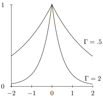
Figure \( 10.4\): \(f(t)=e^{-|\Gamma t|}\) for \(\Gamma=0.5\) and \(\Gamma=2\).

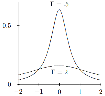
Figure \( 10.5\): \(C(\omega)\) for the same values of \(\Gamma\).

Broad Generalities

We can state this fact very generally using a precise mathematical definition of the spread of the signal in time and the spread of the spectrum in frequency.

We will define the intensity of the signal to be proportional to \(|f(t)|^{2}\). Then, we can define the average value of any function \(g(t)\) weighted with the signal’s intensity as follows \[\langle g(t)\rangle=\frac{\int_{-\infty}^{\infty} d t g(t)|f(t)|^{2}}{\int_{-\infty}^{\infty} d t|f(t)|^{2}} .\]

This weights \(g(t)\) most when the signal is most intense.

For example, \(\langle t\rangle\) is the average time, that is the time value around which the signal is most intense. Then \[\left\langle[t-\langle t\rangle]^{2}\right\rangle \equiv \Delta t^{2}\]

measures the mean-square deviation from the average time, so it is a measure of the spread of the signal.

We can define the average value of a function of \(\omega\) in an analogous way by integrating over the intensity of the frequency spectrum. But here is the trick. Because of (10.9) and (10.37), we can go back and forth between \(f(t)\) and \(C(\omega)\) at will. They carry the same information. We ought to be able to calculate averages of functions of \(\omega\) by using an integral over \(t\). And sure enough, we can. Consider the integral \[\int_{-\infty}^{\infty} d \omega \omega C(\omega) e^{-i \omega t}=i \frac{\partial}{\partial t} \int_{-\infty}^{\infty} d \omega C(\omega) e^{-i \omega t}=i \frac{\partial}{\partial t} f(t) .\]

This shows that multiplying \(C(\omega)\) by \(\omega\) is equivalent to differentiating the corresponding \(f(t)\) and multiplying by \(i\).

Thus we can calculate \(\langle\omega\rangle\) as \[\langle\omega\rangle=\frac{\int_{-\infty}^{\infty} d t f(t)^{*} i \frac{\partial}{\partial t} f(t)}{\int_{-\infty}^{\infty} d t|f(t)|^{2}} ,\]

and \[\Delta \omega^{2} \equiv\left\langle[\omega-\langle\omega\rangle]^{2}\right\rangle=\frac{\int_{-\infty}^{\infty} d t\left|\left(i \frac{\partial}{\partial t}-\langle\omega\rangle\right) f(t)\right|^{2}}{\int_{-\infty}^{\infty} d t|f(t)|^{2}} .\]

\(\Delta \omega\) is a measure of the spread of the frequency spectrum, or the “bandwidth.”

Now we can state and prove the following result: \[\Delta t \cdot \Delta \omega \geq \frac{1}{2} .\]

One important consequence of this theorem is that for a given bandwidth, \(\Delta \omega\), the spread in time of the signal cannot be arbitrarily small, but is bounded by \[\Delta t \geq \frac{1}{2 \Delta \omega} .\]

The smaller the minimum possible value of \(\Delta t\) you can send, the higher the “fidelity” you can achieve. Smaller \(\Delta t\) means that you can send signals with sharper details. But (10.63) means that the smaller the bandwidth, the larger the minimum \(\Delta t\), and the lower the fidelity.

To prove (10.62) consider the function³ \[\left([t-\langle t\rangle]-i \kappa\left[i \frac{\partial}{\partial t}-\langle\omega\rangle\right]\right) f(t)=r(t),\]

which depends on the entirely free parameter \(\kappa\). Now look at the ratio \[\frac{\int_{-\infty}^{\infty} d t|r(t)|^{2}}{\int_{-\infty}^{\infty} d t|f(t)|^{2}} .\]

This ratio is obviously positive, because the integrands of both the numerator and the denominator are positive. What we will do is choose \(\kappa\) cleverly, so that the fact that the ratio is positive tells us something interesting.

First, we will simplify (10.65). In the terms in (10.65) that involve derivatives of \(f(t)^{*}\), we can integrate by parts (and throw away the boundary terms because we assume \(f(t)\) goes to zero at infinity) so that the derivatives act on \(f(t)\). Then (10.65) becomes \[\Delta t^{2}+\kappa^{2} \Delta \omega^{2}+\kappa \frac{\int_{-\infty}^{\infty} d t f(t)^{*}\left(t \frac{\partial}{\partial t}-\frac{\partial}{\partial t} t\right) f(t)}{\int_{-\infty}^{\infty} d t|f(t)|^{2}} .\]

All other terms cancel. But \[\frac{\partial}{\partial t}[t f(t)]=f(t)+t \frac{\partial}{\partial t} f(t) .\]

Thus the last term in (10.66) is just \(\kappa\), and (10.65) becomes \[\Delta t^{2}+\kappa^{2} \Delta \omega^{2}-\kappa .\]

(10.68) is clearly greater than or equal to zero for any value of \(\kappa\), because it is a ratio of positive integrals. To get the most information from the fact that it is positive, we should choose \(\kappa\) so that (10.65) (=(10.68)) is as small as possible. In other words, we should find the value of \(\kappa\) that minimizes (10.68). If we differentiate (10.68) and set the result to zero, we find \[\kappa_{\min }=\frac{1}{2 \Delta \omega^{2}} .\]

We can now plug this back into (10.68) to find the minimum, which is still greater than or equal to zero. It is \[\Delta t^{2}-\frac{1}{4 \Delta \omega^{2}} \geq 0\]

which immediately yields (10.62).

Equation (10.62) appears in many places in physics. A simple example is bandwidth in AM radio transmissions. A typical commercial AM station broadcasts in a band of frequency about 5000 cycles/s (5 kc) on either side of the carrier wave frequency. Thus \[\Delta \omega=2 \pi \Delta \nu \approx 3 \times 10^{4} \mathrm{~s}^{-1} ,\]

and they cannot send signals that separate times less than a few \(\times 10^{-5}\) seconds apart. This is good enough for talk and acceptable for some music.

A famous example of (10.62) comes from quantum mechanics. There is a completely analogous relation between the spatial spread of a wave packet, \(\Delta x\), and the spread of \(k\) values required to produce it, \(\Delta k\): \[\Delta x \cdot \Delta k \geq \frac{1}{2}\]

In quantum mechanics, the momentum of a particle is related to the \(k\) value of the wave that describes it by \[p=\hbar k ,\]

where \(\hbar\) is Planck’s constant \(h\) divided by \(2 \pi\). Thus (10.72) implies \[\Delta x \cdot \Delta p \geq \frac{\hbar}{2} .\]

This is the mathematical statement of the fact that the position and momentum of a particle cannot be specified simultaneously. This is Heisenberg’s uncertainty relation.

___________________
²A example of a physical system with this kind of boundary condition would be a string stretched around a frictionless cylinder with radius \(\ell\) and (therefore) circumference \(2 \pi \ell\). Then (10.42) would be true because \(x=-\pi \ell\) describes the same point on the string as \(x=\pi \ell\).
³This is a trick borrowed from a similar analysis that leads to the Heisenberg uncertainty principle in quantum mechanics. Don’t worry if it is not obvious to you where it comes from. The important thing is the result.