12.1: The String in Three Dimensions

In most of our discussions of wave phenomena so far, we have assumed that the motion is taking place in a plane, so that we can draw pictures of the system on a sheet of paper. We have implicitly been restricting ourselves to two-dimensional waves. This is all right for longitudinal oscillations in three dimensions, because all the action is taking place along a single line. However, for transverse oscillations, going from two dimensions to three dimensions makes an enormous difference because there are two transverse directions in which the system can oscillate.

For example, consider a string in three dimensions, stretched in the \(z\) direction. Each point on the string can oscillate in both the \(x\) direction and the \(y\) direction. If the system were not approximately linear, this could be a horrendous problem. Linearity allows us to solve the problem of oscillation in the \(x\)-\(z\) plane separately from the problem of oscillation in the \(y\)-\(z\) plane. We have already solved these two-dimensional problems in chapter 5. Then we can simply put the results together to get the most general motion of the three-dimensional system. In other words, we can treat the \(x\) component of the transverse oscillation and the \(y\) component as completely independent.

Suppose that there is a harmonic traveling wave in the +\(z\) direction in the string. The displacement of the string at \(z\) from its equilibrium position, \((0, 0, z)\), can be written as \[\vec{\Psi}(z, t)=\operatorname{Re}\left[\left(\psi_{1} \hat{x}+\psi_{2} \hat{y}\right) e^{i(k z-\omega t)}\right]\]

where \(\hat{x}\) and \(\hat{y}\) are unit vectors in the \(x\) and \(y\) direction and \(\psi_{1}\) and \(\psi_{2}\) are complex parameters describing the amplitude and phase of the oscillations in the \(x\)-\(z\) plane and the \(y\)-\(z\) plane, \[\psi_{j}=A_{j} e^{i \phi_{j}} \text { for } j=1 \text { to } 2.\]

It is convenient to arrange these parameters into a complex vector \[Z=\left(\begin{array}{l}
\psi_{1} \\
\psi_{2}
\end{array}\right) ,\]

which gives a complete description of the motion of the string.

Polarization

12-1

“Polarization” refers to the nature of the motion of a point on the string (or other transverse oscillation). This motion is animated in program 12-1. You may want to read the discussion below with this program running.

If \(\phi_{1}=\phi_{2}\), or \(A_{1}\) or \(A_{2}\) is zero, then (12.3) represent a linearly polarized string. Linear polarization is easy to understand. It means that each point on the string is oscillating back and forth in a fixed plane. For example, \[u_{1}=\left(\begin{array}{l}
1 \\
0
\end{array}\right)\]
\[u_{2}=\left(\begin{array}{l}
0 \\
1
\end{array}\right)\]

represent strings oscillating in the \(x\)-\(z\) plane and the \(y\)-\(z\) plane respectively. A string oscillating in a plane an angle \(\theta\) from the positive \(x\) axis (towards the positive \(y\) axis) is represented by \[u_{\theta}=\left(\begin{array}{l}
\cos \theta \\
\sin \theta
\end{array}\right) .\]

This is shown in the \(x\)-\(y\) plane in Figure \( 12.1\). The polarization vectors (12.4)-(12.6) can be multiplied by a phase factor, \(e^{i \phi}\), without affecting the polarization state in any important way. This just corresponds to an overall resetting of the clock.

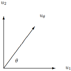
Figure \( 12.1\): \(u_{1}\), \(u_{2}\) and \(u_{\theta}\).

More interesting is circular polarization. A circularly polarized wave in a string is represented by either \[\left(\begin{array}{l}
1 \\
i
\end{array}\right)\]

or \[\left(\begin{array}{c}
1 \\
-i
\end{array}\right) .\]

In (12.7), the \(y\) component lags behind the \(x\) component by \(\pi / 2\left(=\phi_{2}\right)\). Thus, at any fixed point in space, the field rotates from \(x\) to \(y\), or in the counterclockwise direction viewed from the positive \(z\) axis (with the wave coming at you), as shown in Figure \( 12.2\). This is called “left-circular polarization” because the string resembles a left-handed screw. Likewise, \[\left(\begin{array}{c}
1 \\
-i
\end{array}\right) .\]

represents clockwise rotation of the string. This is called “right-circular polarization.”

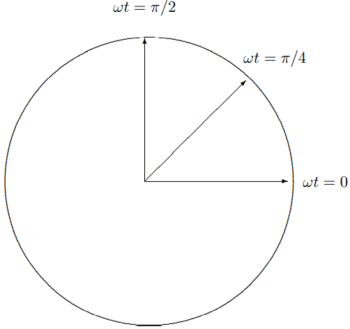
Figure \( 12.2\): Circular polarization.

The vector \[\left(\begin{array}{c}
A \\
i B
\end{array}\right)\]

with \(A > B > 0\) represents elliptical polarization. A point on the string traces out an ellipse with semi-major axis \(A\) along the 1 axis and semi-minor axis \(B\) along the 2 axis, with counterclockwise rotation, as shown in Figure \( 12.3\)

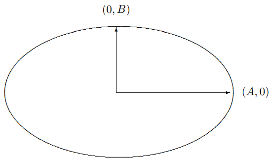
Figure \( 12.3\): Elliptical polarization with long axis in the \(x\) direction.

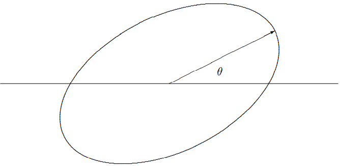
Figure \( 12.4\): General elliptical polarization.

A completely general vector can be written in the following form: \[\left(\begin{array}{l}
\psi_{1} \\
\psi_{2}
\end{array}\right)=e^{i \phi}\left(\begin{array}{c}
A \cos \theta-i B \sin \theta \\
A \sin \theta+i B \cos \theta
\end{array}\right)\]

with \(A \geq|B|\) and \(0 \leq \theta<\pi\) and \(\phi\) is real phase (which is not very relevant relevant to the physics but can be there to make the math look uglier). This represents elliptical polarization with semi-major axis \(A\) at an angle \(\theta\) with the 1 axis, as in \[u_{\theta}=\left(\begin{array}{c}
\cos \theta \\
\sin \theta
\end{array}\right) .\]

and semi-minor axis \(B\) as shown in Figure \( 12.4\). If \(B\) is positive (negative), the rotation is counterclockwise (clockwise). The physically interesting parameters \(A\), \(B\) and \(\theta\) can be found from \(\psi_{1}\) and \(\psi_{2}\) as follows: \[\begin{gathered}
A^{2}+B^{2}=\left|\psi_{1}\right|^{2}+\left|\psi_{2}\right|^{2} , \\
A B=-\operatorname{Im}\left(\psi_{1} \psi_{2}^{*}\right) .
\end{gathered}\]

Thus, \[A \pm B=\sqrt{\left|\psi_{1}\right|^{2}+\left|\psi_{2}\right|^{2} \mp 2 \operatorname{Im}\left(\psi_{1} \psi_{2}^{*}\right)} ,\]

gives \(A\) and \(B\). Then \(\theta\) satisfies \[\begin{aligned}
&\left(A^{2}-B^{2}\right) \cos 2 \theta=\left|\psi_{1}\right|^{2}-\left|\psi_{2}\right|^{2} , \\
&\left(A^{2}-B^{2}\right) \sin 2 \theta=2 \operatorname{Re}\left(\psi_{1} \psi_{2}^{*}\right) .
\end{aligned}\]

Notice that the overall phase factor \(e^{i \phi}\) cancels out in (12.11)-(12.13).