12.5: Radiation

In this section, we write down the electric and magnetic fields associated with changing charge and current densities.

Fields of moving charges

Because Maxwell’s equations are partial differential equations, lots of initial conditions or boundary conditions must be specified to determine the solutions. For example, a constant electric field everywhere is a solution to the free-space Maxwell’s equations, and therefore you can add a constant field to any solution and it will still be a solution. Such things must be determined by physical initial conditions or boundary conditions. One set of conditions that is frequently interesting is an analog of the boundary condition at infinity that we discussed for one-dimensional waves. Suppose that you have a universe which is initially stationary, with no electric currents, no magnetic fields, and only electric fields due to stationary charges (which you know how to compute from Physics 15b). At some time, you begin to move charges around in some finite region of space. What are the electric and magnetic fields produced in this way? This question has a relatively simple answer that is a nice intuitive generalization of the relations you learned in 15b for the electric and vector potentials from stationary charge and current distributions. These relations were \[\phi(\vec{r})=\int d^{3} r^{\prime} \frac{\rho\left(\vec{r}^{\prime}\right)}{\left|\vec{r}-\overrightarrow{r^{\prime}}\right|}\]

\[\vec{A}(\vec{r})=\frac{1}{c} \int d^{3} r^{\prime} \frac{\overrightarrow{\mathcal{J}}\left(\vec{r}^{\prime}\right)}{\left|\vec{r}-\overrightarrow{r^{\prime}}\right|}\]

The generalizations are \[\phi(\vec{r}, t)=\int d^{3} r^{\prime} \frac{\rho\left(\overrightarrow{r^{\prime}}, t-\left|\vec{r}-\vec{r}^{\prime}\right| / c\right)}{\left|\vec{r}-\vec{r}^{\prime}\right|}\]

\[\vec{A}(\vec{r}, t)=\frac{1}{c} \int d^{3} r^{\prime} \frac{\overrightarrow{\mathcal{J}}\left(\overrightarrow{r^{\prime}}, t-|\vec{r}-\vec{r}| / c\right)}{\left|\vec{r}-\overrightarrow{r^{\prime}}\right|}\]

It is a straightforward, but tedious, exercise in vector calculus to show these satisfy Maxwell’s equations. I am not going to talk about this (I’ll write down the derivation in an appendix for those of you who are interested), but it is worth trying to understand what these relations mean physically. The important physical point that these relations imply is that if the charge and current distributions depend on time, and if they are producing the fields, then what determines what the field is at some point \(\vec{r}\) is the values of the charge and current distributions at earlier times. The farther away the charge is, the earlier the time has to be. That is what the factor of \(t-\left|\vec{r}-\vec{r}^{\prime}\right| / c\) is telling us. The appearance of this factor is a kind of boundary condition at infinity. It is consistent with the relativistic version of the principle of causality. Because information cannot be transferred faster than light, a charge distribution at a space-time point \(\left(\vec{r}^{\prime}, t^{\prime}\right)\) can effect the fields at the space-time point \((\vec{r}, t)\), only if \(t \geq t^{\prime}\) and \[\frac{\left|\vec{r}-\vec{r}^{\prime}\right|}{t-t^{\prime}} \leq c\]

In these relations, (12.82) and (12.83), however, the condition is even stronger — a charge distribution at a space time point \(\left(\vec{r}^{\prime}, t^{\prime}\right)\) can effect the fields at the space time point \((\vec{r}, t)\) only if light can travel directly from \(\left(\vec{r}^{\prime}, t^{\prime}\right)\) to \((\vec{r}, t)\) — that is if\(t \geq t^{\prime}\) and \[\text { ck }\]

or \[t-t^{\prime}=\left|\vec{r}-\overrightarrow{r^{\prime}}\right| / c\]

or \[t^{\prime}=t-\left|\vec{r}-\vec{r}^{\prime}\right| / c\]

These are just words. We have not derived this! The real justification of this discussion comes when you check that the relations actually satisfy Maxwell’s equations. That can wait for Physics 153 or 232 (or the appendix if you are in a hurry). However, I hope that this discussion at least makes the result reasonable. In fact you have already seen the result in action in 15b in Purcell’s discussion of the electric field from a charge that starts and stops. Look at the ANIMATIONS - PURCELL - the field from a charge that suddenly accelerates. This is an animation of a famous figure in Purcell’s book. The interesting thing about the animation is the kink in the electric field that propagates out from the acceleration event at the velocity of light — because it is light. Inside the kink, the fields are those of the moving charge. Outside the kind, the fields are those of the stationary charge. The kink — the electromagnetic way — is what connects the two asymptotic regions together. It is also fun to compare with PURCELL2 which illustrates what happens if an initially moving charge stops suddenly.

Now let’s see at what the electric and magnetic fields look like in an important limit. The connection between the potentials and the fields is the following: \[\vec{E}=-\vec{\nabla} \phi-\frac{1}{c} \frac{\partial}{\partial t} \vec{A}\]

\[\vec{B}=\vec{\nabla} \times \vec{A}\]

These relations are completely general. The special limit that I want to consider is one in which the charges and currents are confined to a small region around \(\vec{r} = 0\). Then we will look at the electric and magnetic fields produced by the moving charges far away, for large \(|\vec{r}|\). It is actually easiest to look at the magnetic field: \[\vec{B}=\vec{\nabla} \times \vec{A}=\vec{\nabla} \times \frac{1}{c} \int d^{3} r^{\prime} \frac{\overrightarrow{\mathcal{J}}\left(\overrightarrow{r^{\prime}}, t-\left|\vec{r}-\vec{r}^{\prime}\right| / c\right)}{\left|\vec{r}-\vec{r}^{\prime}\right|}\]

The point is that the curl \((\vec{\nabla} \times)\) can operate in two different places, either on the \(1 /\left|\vec{r}-\overrightarrow{r^{\prime}}\right|\) or on the \(-\left|\vec{r}-\overrightarrow{r^{\prime}}\right| / c\) in the time dependence of \(\mathcal{J}\). The first gives a contribution that drops of like \(1 / r^{2}\) for large \(r\), just like the magnetic field from a time-independent distribution of currents. But the second gives a contribution that only falls off like \(1/r\). Thus this contribution dominates for large \(r\). Explicitly (using the chain rule), it is \[\vec{B}=-\frac{1}{c^{2}} \int d^{3} r^{\prime} \frac{\vec{r}-\vec{r}^{\prime}}{\left|\vec{r}-\vec{r}^{\prime}\right|^{2}} \times \frac{d}{d t} \overrightarrow{\mathcal{J}}\left(\vec{r}^{\prime}, t-\left|\vec{r}-\vec{r}^{\prime}\right| / c\right)\]

\[\rightarrow-\frac{1}{c^{2}} \frac{1}{r} \int d^{3} r^{\prime} \hat{r} \times \frac{d}{d t} \overrightarrow{\mathcal{J}}\left(\overrightarrow{r^{\prime}}, t-\left|\vec{r}-\vec{r}^{\prime}\right| / c\right)\]

where in (12.92) we have dropped a \(\overrightarrow{r^{\prime}}\) in the numerator because this term falls like \(1 / r^{2}\) for large \(r\).

This is the magnetic field of an electromagnetic wave. Notice that it is perpendicular to the direction of motion \((\hat{r})\). The \(1/r\) fall-off is what we expect for an electromagnetic wave, because the energy density goes like the square of the field, and falls off like \(1 / r^{2}\) as the wave spreads.

The electric field can be computed in a similar way, although you also need to use the conservation of electric charge. \[\frac{\partial}{\partial t} \rho+\vec{\nabla} \cdot \overrightarrow{\mathcal{J}}=0\]

As you would expect, the result is that the electric field has the same magnitude as the magnetic field and is perpendicular to both direction of motion and to the magnetic field. The piece that corresponds to a traveling electromagnetic wave can be written as \[\vec{E} \rightarrow-\frac{1}{c^{2}} \int d^{3} r^{\prime} \frac{\vec{r}-\overrightarrow{r^{\prime}}}{\left|\vec{r}-\overrightarrow{r^{\prime}}\right|} \times\left(\frac{\vec{r}-\overrightarrow{r^{\prime}}}{\left|\vec{r}-\overrightarrow{r^{\prime}}\right|^{2}} \times \frac{d}{d t} \overrightarrow{\mathcal{J}}\left(\overrightarrow{r^{\prime}}, t-\left|\vec{r}-\vec{r}^{\prime}\right| / c\right)\right)\]

\[\rightarrow \frac{1}{c^{2}} \frac{1}{r} \int d^{3} r^{\prime} \hat{r} \times\left(\hat{r} \times \frac{d}{d t} \overrightarrow{\mathcal{J}}\left(\overrightarrow{r^{\prime}}, t-\left|\vec{r}-\vec{r}^{\prime}\right| / c\right)\right)\]

To lowest order in \(1/r\) for charges moving with velocities much smaller than \(c\), we can simplify the electric field in (12.95) by substituting \[|\vec{r}-\vec{r}| \rightarrow r\]

and write the result as \[\vec{E}(\vec{r}, t) \approx \frac{1}{c^{2}} \frac{1}{r} \int d^{3} r^{\prime} \hat{r} \times\left(\hat{r} \times \frac{d}{d t} \overrightarrow{\mathcal{J}}\left(\overrightarrow{r^{\prime}}, t-r / c\right)\right)\]

The reason for the restriction to nonrelativistic motion of charges is that if a charged particle is moving at a speed close to the velocity of light, then we cannot neglect its position, \(\overrightarrow{r^{\prime}}\), when it is moving towards \(\vec{r}\). To see this, consider the impossible limit in which the charge is moving towards the point \(\vec{r}\) at the speed of light. Then if the charge contributes to the electric field at \(\vec{r}\) at one time, then it also contributes at later times because the particle keeps up with the moving light wave. While \(v = c\) is impossible, for \(v \approx c\), the \(\overrightarrow{r^{\prime}}\) dependence cannot be ignored because it leads to very rapid time dependence of the potentials, and hence to large fields. What happens is that the contribution of charges moving relativistically to the electric fields in front of them get enhanced by factors of \(\frac{c}{c-v}\). This effect is widely used today to produce intense “light” from particle accelerators — so called synchrotron radiation. You can see this effect in the ANIMATIONS if you make \(v\) close to 1.

A particularly important and instructive case of (12.97) is the nonrelativistic motion of a single charge, \(Q\), moving along a trajectory \(\vec{R}(t)\). For this system,⁵ \[\overrightarrow{\mathcal{J}}(\vec{r}, t)=Q \vec{v}(t) \delta^{3}(\vec{r}-\vec{R}(t))=Q \frac{d \vec{R}(t)}{d t} \delta^{3}(\vec{r}-\vec{R}(t))\]

Then the integration over \(d^{3} r^{\prime}\) in \((a)\) eliminates the \(\delta\)-function, and the electric field of the outgoing electromagnetic wave is proportional to the acceleration, \[\vec{E}(\vec{r}, t) \approx \frac{1}{c^{2}} \frac{1}{r} Q \hat{r} \times(\hat{r} \times \vec{a}(t-r / c))\]

where \[\vec{a}(t)=\frac{d^{2} \vec{R}(l)}{d t^{2}}\]

All that the cross products with \(\hat{r}\) do is to pick out minus the component of \(\vec{a}(l-r / c)\) that is perpendicular to \(\vec{r}\). It follows from the famous “bac-cab” identity, \[\vec{a} \times(\vec{b} \times \vec{c})=\vec{b}(\vec{a} \cdot \vec{c})-\vec{c}(\vec{a} \cdot \vec{b}),\]

that \[\vec{E}(\vec{r}, t) \approx-\frac{1}{c^{2}} \frac{1}{r} Q(\vec{a}(t-r / c)-\hat{r}(\hat{r} \cdot \vec{a}(t-r / c))) .\]

This had to happen because the electric field of an electromagnetic wave is perpendicular to its direction of motion. In this case, for large \(r\), the wave is nearly a plane wave moving in direction \(\vec{r}\).

Antenna Pattern

Let us do an even more explicit example by considering a charge that oscillates harmonically along the \(z\) axis, \[\vec{R}(t)=\ell \hat{z} \cos \omega t .\]

so that \[\vec{a}(t)=-\ell \omega^{2} \hat{z} \cos \omega t .\]

\[\vec{E}(\vec{r}, t) \approx \frac{\ell \omega^{2}}{c^{2}} \frac{1}{r} Q(\hat{z}-\hat{r}(\hat{r} \cdot \hat{z})) \cos [\omega(t-r / c)] .\]

The vector \(\hat{z}-\hat{r}(\hat{r} \cdot \hat{z})\) is the component of \(\hat{z}\) perpendicular to \(\vec{r}\), as illustrated in Figure \( 12.13\).

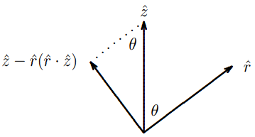
Figure \( 12.13\):

Evidently, the magnitude of \(\hat{z}-\hat{r}(\hat{r} \cdot \hat{z})\) is \(\sin \theta\). This means that the intensity of the electromagnetic wave at an angle \(\theta\) from the \(z\) axis is proportional to \(\sin ^{2} \theta\). The intensity pattern can be conveniently represented in polar coordinates, where we plot the intensity as a function of \(\theta\). The result is shown below. This is the “antenna pattern” for the oscillating

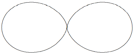
Figure \( 12.14\):

dipole in the \(z\) direction. It is shown in Figure \( 12.14\). The two lobes of the pattern arise because the field is highest in the \(x\)-\(y\) plane, for \(\theta=\pi / 2\), and drops to zero as we approach the \(z\) axis, \(\theta = 0\) or \(\theta = \pi\).

Checking Maxwell’s equations

These things are called retarded potentials. This is a confusing name, since there is really nothing special about the potentials themselves. What is special is the assumption of a particular relation between the potentials and the charges and currents — that the fields are being produced entirely by the charges and currents. Here I show that they satisfy Maxwell’s equations. I call this an appendix because you are NOT responsible for knowing the details. I include it for your general education.

Some mathematical things to notice about the solution: \[\frac{\partial}{\partial t} \rho+\vec{\nabla} \cdot \overrightarrow{\mathcal{J}}=0\]

implies \[\frac{\partial}{\partial t} \rho+\vec{\nabla} \cdot \overrightarrow{\mathcal{J}}=0\]

This is called the Lorentz gauge condition. \[\vec{\nabla} \cdot \vec{E}=-\nabla^{2} \phi-\frac{1}{c} \frac{\partial}{\partial t} \vec{\nabla} \cdot \vec{A}\]

\[=\left(-\nabla^{2}+\frac{1}{c^{2}} \frac{\partial^{2}}{\partial t^{2}}\right) \phi\]

\[=\int d^{3} r^{\prime}\left(\rho\left(\overrightarrow{r^{\prime}}, t-\left|\vec{r}-\vec{r}^{\prime}\right| / c\right)\left(-\nabla^{2}\right) \frac{1}{\left|\vec{r}-\overrightarrow{r^{\prime}}\right|}\right.\]

\[+\frac{1}{\left|\vec{r}-\vec{r}^{\prime}\right|}\left(-\nabla^{2}+\frac{1}{c^{2}} \frac{\partial^{2}}{\partial t^{2}}\right) \rho\left(\overrightarrow{r^{\prime}}, t-\left|\vec{r}-\vec{r}^{\prime}\right| / c\right)\]

\[\left.-2\left(\vec{\nabla} \rho\left(\overrightarrow{r^{\prime}}, t-\left|\vec{r}-\vec{r}^{\prime}\right| / c\right)\right) \cdot\left(\vec{\nabla} \frac{1}{\left|\vec{r}-\overrightarrow{r^{\prime}}\right|}\right)\right)\]

The first term is the one we want. It is \[=\int d^{3} r^{\prime} \rho\left(\vec{r}^{\prime}, t-\left|\vec{r}-\vec{r}^{\prime}\right| / c\right) 4 \pi \delta^{3}\left(\vec{r}-\vec{r}^{\prime}\right)\]

\[=4 \pi \rho(\vec{r}, t)\]

The other two terms cancel because of the special form of the variable \(t-\left|\vec{r}-\overrightarrow{r^{\prime}}\right| / c\). \[\frac{1}{\left|\vec{r}-\overrightarrow{r^{\prime}}\right|}\left(-\nabla^{2}+\frac{1}{c^{2}} \frac{\partial^{2}}{\partial t^{2}}\right) \rho\left(\vec{r}^{\prime}, t-\left|\vec{r}-\vec{r}^{\prime}\right| / c\right)\]

\[-2\left(\vec{\nabla} \rho\left(\overrightarrow{r^{\prime}}, t-\left|\vec{r}-\vec{r}^{\prime}\right| / c\right)\right) \cdot\left(\vec{\nabla} \frac{1}{\left|\vec{r}-\vec{r}^{\prime}\right|}\right)\]

\[=\frac{1}{\left|\vec{r}-\vec{r}^{\prime}\right|} \frac{1}{c^{2}} \ddot{\rho}\left(\vec{r}^{\prime}, t-\left|\vec{r}-\vec{r}^{\prime}\right| / c\right)\]

\[+\frac{1}{\left|\vec{r}-\vec{r}^{\prime}\right|} \frac{1}{c} \vec{\nabla} \cdot \frac{\vec{r}-\vec{r}^{\prime}}{\left|\vec{r}-\vec{r}^{\prime}\right|} \dot{\rho}\left(\overrightarrow{r^{\prime}}, t-\left|\vec{r}-\vec{r}^{\prime}\right| / c\right)\]

\[-2 \frac{1}{c} \frac{1}{\left|\vec{r}-\vec{r}^{\prime}\right|} \dot{\rho}\left(\vec{r}^{\prime}, t-\left|\vec{r}-\vec{r}^{\prime}\right| / c\right)\]

where \(*\) means differentiation with respect to the time variable: \[\left.\dot{\rho}\left(\overrightarrow{r^{\prime}}, t-\left|\vec{r}-\vec{r}^{\prime}\right| / c\right) \equiv \frac{\partial}{\partial t^{\prime}} \rho\left(\overrightarrow{r^{\prime}}, t^{\prime}\right)\right|_{t^{\prime}=t-\left|\vec{r}-\vec{r}^{\prime}\right| / c}\]

\(i\) and \(ii\) come from \(a\) (from the \(\frac{\partial^{2}}{\partial t^{2}}\) and \(−\nabla^{2}\) terms respectively) and \(iii\) comes from \(b\). Now the \(\vec{\nabla}\) in \(ii\) gives two terms — acting on \(\dot{\rho}\) cancels \(i\) and acting on cancels \(iii\). Thus \[\vec{\nabla} \cdot \vec{E}=4 \pi \rho .\]

Likewise, \[\vec{\nabla} \times \vec{B}-\frac{1}{c} \frac{\partial}{\partial t} \vec{E}\]

\[=\vec{\nabla} \times(\vec{\nabla} \times \vec{A})-\frac{1}{c} \frac{\partial}{\partial t}\left(-\vec{\nabla} \phi-\frac{1}{c} \frac{\partial}{\partial t} \vec{A}\right)\]

\[=\vec{\nabla}(\vec{\nabla} \cdot \vec{A})-\nabla^{2} \vec{A}-\vec{\nabla}\left(\frac{1}{c} \frac{\partial}{\partial t} \phi\right)+\frac{1}{c^{2}} \frac{\partial^{2}}{\partial t^{2}} \vec{A}\]

or using the Lorentz gauge condition, \[=\left(-\nabla^{2}+\frac{1}{c^{2}} \frac{\partial^{2}}{\partial t^{2}}\right) \vec{A}\]

Form here on, the derivation is the same as for \(\vec{\nabla} \cdot \vec{E}\), and we find \[\vec{\nabla} \times \vec{B}-\frac{1}{c} \frac{\partial}{\partial t} \vec{E}=\frac{4 \pi}{c} \overrightarrow{\mathcal{J}}\]

QED.

__________________

⁵ This equation makes use of δ-function notation. To a physicist, a δ-function δ(x) is just a function that has area 1 and is so sharply peaked around x = 0 that we don’t care exactly what it looks like. All that matters is the area and where the peak is. The δ3 ~ ¡ ~r − R(t) ¢ in the equation is actually the product of three delta functions, for the x, y and z components, and just tells you that ~r = (x, y, z) = R~(t) = ¡ X(t), Y (t), Z(t) ¢ — that is that the particle is moving along the trajectory R~(t). For a mathematical discussion of the δ-function you can look at http://mathworld.wolfram.com/DeltaFunction.html. But don’t be frightened. It is just a simple device for ignoring small details that we don’t care about. If you translate the integral into words or pictures, it may help.