12.4: Boundary between Dielectrics

Let us return to the infinite plane boundary between two dielectrics that we discussed in chapter 9, but now consider an electromagnetic wave coming in at an arbitrary angle. As in chapter 5, we will assume that the boundary is the $z = 0$ plane, and that for $z < 0$ we have dielectric constant $\epsilon$, while for $z > 0$, dielectric constant $\epsilon^{\prime}$. We assume $\mu=1$ everywhere.

On the general grounds of translation invariance and local interactions discussed in the previous chapter, all the components of the electric and magnetic fields will have the general form $$\begin{array}{cl} \psi(r, t) \propto e^{i \vec{k} \cdot \vec{r}}+R e^{i \vec{k} \cdot \vec{r}} & \text { for } z \leq 0 \\ \psi(r, t) \propto \tau e^{i \vec{k}^{\prime} \cdot \vec{r}} & \text { for } z \geq 0 \end{array}$$

where $$\tilde{k}_{x}=k_{x}, \quad k_{x}^{\prime}=k_{x} ,$$

and $$\begin{gathered} \tilde{k}_{z}=-\sqrt{\omega^{2} / v^{2}-k_{x}^{2}}=-k_{z} \\ k_{z}^{\prime}=\sqrt{\omega^{2} / v^{\prime 2}-k_{x}^{2}} \end{gathered} .$$

Thus Snell’s law is satisfied, with $\theta$ and $\theta^{\prime}$ defined as shown in Figure $12.10$. $$\begin{aligned} &k \cdot \sin \theta=k^{\prime} \sin \theta^{\prime} . \\ &|\vec{k}|=\sqrt{\mu \epsilon} \frac{\omega}{c}=n \frac{\omega}{c} \\ &n \sin \theta=n^{\prime} \sin \theta^{\prime} . \end{aligned}$$

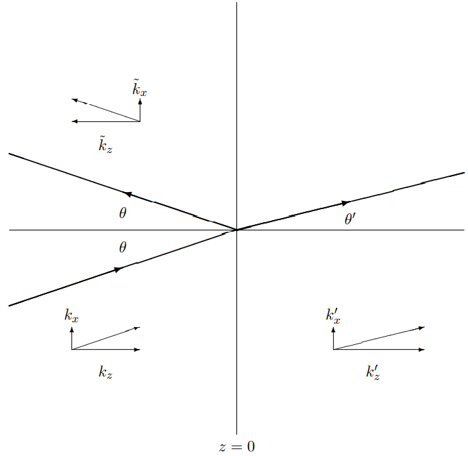
Figure $12.10$: Scattering of plane waves from a plane boundary.

The details of the scattering will depend on the polarization. It is clear (by symmetry as usual) that the two cases will be polarization in the $x$-$z$ plane and polarization perpendicular to the $x$-$z$ plane. Of course, we lose nothing by considering these two separately, because of linearity. Any polarization for the incoming wave can be dealt with by forming a linear combination of the parallel and perpendicular solutions.

Polarization Perpendicular to the Scattering Plane

Let us first consider perpendicular polarization. This means that the electric field is in the $y$ direction (out of the plane of the paper), while the magnetic field is the $x$-$z$ plane:⁴ $$\begin{gathered} E_{y}(r, t)=A e^{i(\vec{k} \vec{r}-\omega t)}+R_{\perp} A e^{i(\tilde{k} \cdot \vec{r}-\omega t)} \quad \text { for } z \leq 0 \\ E_{y}(r, t)=\tau_{\perp} A e^{i\left(\vec{k}^{\prime} \cdot \vec{r}-\omega t\right)} \quad \text { for } z \geq 0 \\ E_{z}=E_{x}=0 \end{gathered}$$

Using (12.19)) $$\vec{B}=\frac{n}{c} \hat{k} \times \vec{E}=\frac{1}{\omega} \vec{k} \times \vec{E} ,$$

we can write $$\begin{array}{rlr} B_{x}(r, t)=-\frac{n}{c} A \cos \theta e^{i(\vec{k} \cdot \vec{r}-\omega t)}+\frac{n}{c} \cos \theta R_{\perp} A e^{i(\vec{k} \cdot \vec{r}-\omega t)} & \text { for } z \leq 0 \\ B_{x}(r, t)--\frac{n^{\prime}}{c} \cos \theta^{\prime} \tau_{\perp} A e^{i\left(\vec{k}^{\prime} \cdot \vec{r}-\omega t\right)} & & \text { for } z \geq 0 \\ B_{z}(r, t)=\frac{n}{c} \sin \theta A e^{i(\vec{k} \cdot \vec{r}-\omega t)}+\frac{n}{c} \sin \theta R_{\perp} A e^{i(\vec{k} \cdot \vec{r}-\omega t)} & & \text { for } z \leq 0 \\ B_{z}(r, t)=\frac{n^{\prime}}{c} \sin \theta^{\prime} \tau_{\perp} A e^{i\left(\vec{k}^{\prime} \cdot \vec{r}-\omega t\right)} & & \text { for } z \geq 0 \\ B_{y}=0 & \end{array}$$

The system is shown in Figure $12.11$. This figure shows the directions of the magnetic fields of the incoming ($\vec{B}_{i}$), reflected ($\vec{B}_{r}$), and transmitted ($\vec{B}_{t}$) component waves in scattering of an electromagnetic plane wave polarized parallel to a plane dielectric boundary. The $\vec{k}$ vectors are shown directly beneath the magnetic fields. The nontrivial boundary conditions are that $E_{y}$ and $B_{x}$ are continuous (the latter because we have assumed $\mu=1$ so there is no sheet of bound current on the boundary). $B_{z}$ is also continuous, but that provides no new information. Thus $$1+R_{\perp}=\tau_{\perp}$$

where $$\xi_{\perp}=\frac{k_{z}^{\prime}}{k_{z}} .$$

Polarization in the Scattering Plane

Polarization in the $x$-$z$ plane looks like $$\begin{array}{cl} B_{y}(r, t)=A e^{i(\vec{k} \cdot \vec{r}-\omega t)}+R_{\|} A e^{i(\vec{k} \cdot \vec{r}-\omega t)} & \text { for } z \leq 0 \\ B_{y}(r, t)=\tau_{\|} A e^{i\left(\vec{k}^{\prime} \cdot \vec{r}-\omega t\right)} & \text { for } z \geq 0 \\ B_{z}=B_{x}=0, & \end{array}$$

where, for convenience, we have defined the reflection and transmission coefficients in terms of the magnetic fields, and $$\begin{array}{rlr} E_{x}(r, t)=\frac{c}{n} \cos \theta A e^{i(\vec{k} \cdot \vec{r}-\omega t)}-\frac{c}{n} \cos \theta R_{\|} A e^{i(-\overrightarrow{\vec{k}} \cdot \vec{r}-\omega t)} & \text { for } z \leq 0 \\ E_{x}(r, t)=\frac{c}{n^{\prime}} \cos \theta^{\prime} \tau_{\|} A e^{i\left(\vec{k}^{\prime} \cdot \vec{r}-\omega t\right)} & & \text { for } z \geq 0 \\ E_{z}(r, t)=-\frac{c}{n} \sin \theta A e^{i(\vec{k} \cdot \vec{r}-\omega t)}-\frac{c}{n} \sin \theta R_{\|} A e^{i(-\tilde{\vec{k}} \cdot \vec{r}-\omega t)} & & \text { for } z \leq 0 \\ E_{z}(r, t)=-\frac{c}{n^{\prime}} \sin \theta^{\prime} \tau_{\|} A e^{i\left(\vec{k}^{\prime} \cdot \vec{r}-\omega t\right)} & & \text { for } z \geq 0 \\ E_{z}=0 . & \end{array}$$

Now the nontrivial boundary conditions are the continuity of $B_{y}$ and $E_{x}$. $E_{z}$ is not continuous because a surface bound charge density builds up on the dielectric boundary. The boundary conditions yield $$1+R_{\|}=\tau_{\|}$$

$$\frac{\cos \theta}{n}\left(1-R_{\|}\right)=\frac{\cos \theta^{\prime}}{n^{\prime}} \tau_{\|}$$

or $$\tau_{\|}=\frac{2}{1+\xi_{\|}}$$

$$R_{\|}=\frac{1-\xi \|}{1+\xi_{\|}}$$

where $$\xi_{\|}=\frac{\cos \theta^{\prime} / n^{\prime}}{\cos \theta / n}=\frac{n^{2} k_{z}^{\prime}}{n^{\prime 2} k_{z}} .$$

One of the interesting things about (12.74) is that when $$\frac{n^{2} k_{z}^{\prime}}{n^{\prime 2} k_{z}}-1$$

there is no reflection. This condition is satisfied for a special angle of incidence called Brewster’s angle. We can understand the significance of Brewster’s angle as follows: $$\text { from Snell's law, } \frac{n^{2}}{n^{\prime 2}}-\frac{\sin ^{2} \theta^{\prime}}{\sin ^{2} \theta}$$

$$\frac{k_{z}^{\prime}}{k_{z}}=\frac{k_{x} / k_{z}}{k_{x}^{\prime} / k_{z}^{\prime}}=\frac{\tan \theta}{\tan \theta^{\prime}}$$

$$\frac{n^{2} k_{z}^{\prime}}{n^{\prime 2} k_{z}}=\frac{\sin \theta^{\prime} \cos \theta^{\prime}}{\sin \theta \cos \theta}=1 .$$

Thus $\sin 2 \theta=\sin 2 \theta^{\prime}$. Because $\theta \neq \theta^{\prime}$ (that would be the trivial situation with no boundary), this means that $$\theta=\pi / 2-\theta^{\prime} .$$

In other words, Brewster’s angle is defined by the condition that the reflected and transmitted plane waves are perpendicular, as shown in the diagram in Figure $12.12$. The relevance of this condition is that the reflected wave can be thought of as being produced by the motion of the charges on the boundary. But if these are moving in a direction perpendicular to the electric field in the would-be reflected wave, then the wave cannot be produced.

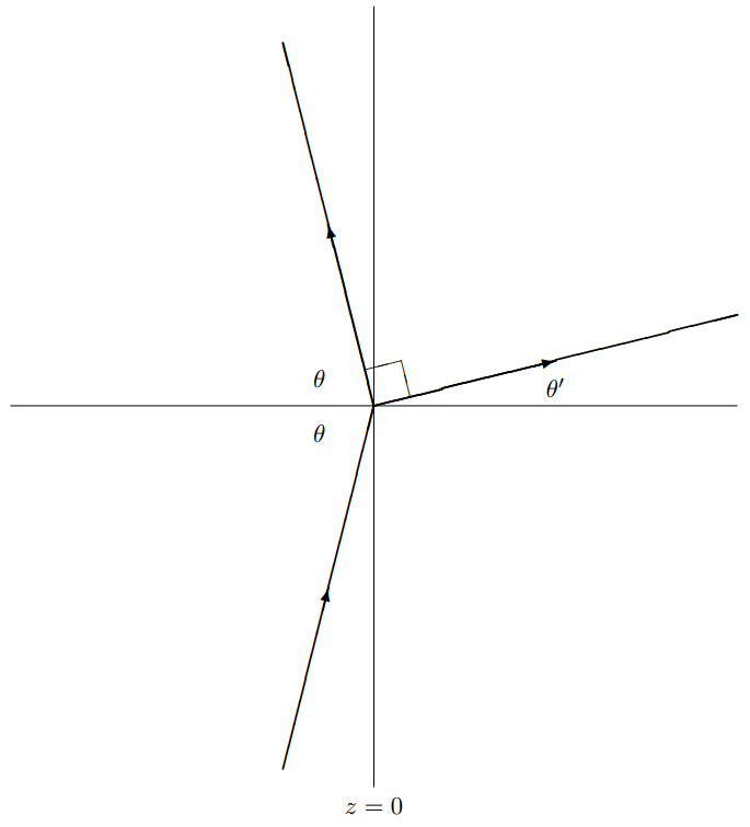
Figure $12.12$: Brewster's angel.

_____________________

⁴ The quantities, $R_{\perp}$ and $\tau_{\perp}$ in this section and $R_{\|}$ and $\tau_{\|}$ in the next are conventionally called “Fresnel coefficients.” See Hecht, page 97.