
3.3: Polarization of Dielectrics


- Last updated
- Mar 5, 2022
- Save as PDF

( \newcommand{\kernel}{\mathrm{null}\,}\)
The general relations derived in the previous section may be used to describe the electrostatics of any dielectrics – materials with bound electric charges (and hence with negligible dc electric conduction). However, to form a full system of equations necessary to solve electrostatics problems, they have to be complemented by certain constitutive relations between the vectors P and E.11
In most materials, in the absence of an external electric field, the elementary dipoles p either equal zero or have a random orientation in space, so that the net dipole moment of each macroscopic volume (still containing many such dipoles) equals zero: P=0 at E=0. Moreover, if the field changes are sufficiently slow, most materials may be characterized by a unique dependence of P on E. Then using the Taylor expansion of function P(E), we may argue that in relatively low electric fields the function should be well approximated by a linear dependence between these two vectors. Such dielectrics are called linear. In an isotropic media, the coefficient of proportionality should be just a scalar. In the SI units, this scalar is defined by the following relation:
Electric susceptibility
P=χeε0E,
with the dimensionless constant χe called the electric susceptibility. However, it is much more common to use, instead of χe, another dimensionless parameter,12
Dielectric constant
κ≡1+χe,
which is sometimes called the “relative electric permittivity”, but much more often, the dielectric constant. This parameter is very convenient, because combining Eqs. (43) and (44),
P=(κ−1)ε0E.
and then plugging the resulting relation into the general Eq. (33), we get simply
D=κε0E, or D=εE,
where another popular parameter,13
Electric permittivity
ε≡κε0≡(1+χe)ε0.
ε is called the electric permittivity of the material.14 Table 1 gives the approximate values of the dielectric constant for several representative materials.
In order to understand the range of these values, let me discuss (rather superficially) the two simplest mechanisms of electric polarization. The first of them is typical for liquids and gases of polar atoms/molecules, which have their own, spontaneous dipole moments p. (A typical example is the water molecule H2O, with the negative oxygen ion offset from the line connecting two positive hydrogen ions, thus producing a spontaneous dipole moment p=ea, with a≈0.38×10⁻¹⁰ m∼rB.) In the absence of an external electric field, the orientation of such dipoles may be random, with the average polarization P=n⟨p⟩ equal to zero – see the top panel of Fig. 7a.
| Material | κ |
|---|---|
| Air (at ambient conditions) | 1.00054 |
| Teflon (polytetrafluoroethylene, [C2 F4]n | 2.1 |
| Silicon dioxide (amorphous) | 3.9 |
| Glasses (of various compositions) | 3.7-10 |
| Castor oil | 4.5 |
| Silicon(a) | 11.7 |
| Water (at 100oC) | 55.3 |
| Water (at 20oC) | 80.1 |
| Barium titanate (BaTiO3, at 20oC) | ~1,600 |
(a) Anisotropic materials, such as silicon crystals, require a susceptibility tensor to give an exact description of the linear relation of the vectors P and E. However, most important crystals (including Si) are only weakly anisotropic, so that they may be reasonably well characterized with a scalar (angle-average) susceptibility.
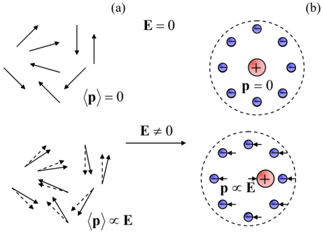
A relatively weak external field does not change the magnitude of the dipole moments significantly, but according to Eqs. (15a) and (17), tries to orient them along the field, and thus creates a non-zero vector average ⟨p⟩ directed along the vector ⟨Em⟩, where Em is the microscopic field at the
point of the dipole’s location – cf. two panels of Fig. 7a. If the field is not two high (p⟨Em⟩<<kBT), the
induced average polarization ⟨p⟩ is proportional to ⟨Em⟩. If we write this proportionality relation in the following traditional form,
Atomic polarizability
⟨p⟩=αEm
where α is called the atomic (or, sometimes, “molecular”) polarizability, this means that α is positive. If the concentration n of such elementary dipoles is low, the contribution of their own fields into the microscopic field acting on each dipole is negligible, and we may identify ⟨Em⟩ with the macroscopic field E. As a result, the second of Eqs. (27) yields
P≡n⟨p⟩=αnE.
Comparing this relation with Eq. (45), we get
κ=1+αε0n,
so that κ>1 (i.e. χe>0). Note that at this particular polarization mechanism (illustrated on the lower panel of Fig. 7a), the thermal motion “tries” to randomize the dipole orientation, i.e. reduce its ordering by the field, so that we may expect α, and hence χe≡κ−1 to increase as temperature T is decreased – the so-called paraelectricity. Indeed, the basic statistical mechanics15 shows that in this case, the electric susceptibility follows the law χe∝1/T.
The materials of the second, much more common class consist of non-polar atoms without intrinsic spontaneous polarization. A crude classical image of such an atom is an isotropic cloud of negatively charged electrons surrounding a positively charged nucleus – see the top panel of Fig. 7b. The external electric field shifts the positive charge in the direction of the vector E, and the negative charges in the opposite direction, thus creating a similarly directed average dipole moment ⟨p⟩.16 At relatively low fields, this average moment is proportional to E, so that we again arrive at Eq. (48), with α>0, and if the dipole concentration n is sufficiently low, also at Eq. (50), with κ−1>0. So, the dielectric constant is larger than 1 for both polarization mechanisms – please have one more look at Table 1.
In order to make a crude but physically transparent estimate of the difference κ−1, let us consider the following toy model of a non-polar dielectric: a set of similar conducting spheres of radius R, distributed in space with a low density n<<1/R3. At such density, the electrostatic interaction of the spheres is negligible, and we can use Eq. (11) for the induced dipole moment of a single sphere. Then the polarizability definition (48) yields α=4πε0R3, so that Eq. (50) gives
κ=1+4πR3n.
Let us use this result for a crude estimate of the dielectric constant of air at the so-called ambient conditions, meaning the normal atmospheric pressure P=1.013×10⁵ Pa and temperature T=300 K. At these conditions the molecular density n may be, with a few-percent accuracy, found from the equation of state of an ideal gas:17 n≈P/kBT≈(1.013×105)/(1.38×10−23×300)≈2.45×1025 m−3. The molecule of the air’s main component, N2, has a van-der-Waals radius18 of 1.55×10⁻¹⁰ m. Taking this radius for the R of our crude model, we get χe≡κ−1≈1.15×10⁻³. Comparing this number with the first line of Table 1, we see that the model gives a surprisingly reasonable result: to get the experimental value, it is sufficient to decrease the effective R of the sphere by just ∼30%, to ∼1.2×10⁻¹⁰ m.19
This result may encourage us to try using Eq. (51) for a larger density n. For example, as a crude model for a non-polar crystal, let us assume that the conducting spheres form a simple cubic lattice with the period a=2R (i.e., the neighboring spheres virtually touch). With this, n=1/a3=1/8R3 and Eq. (44) yields κ=1+4π/8≈2.5. This estimate provides a reasonable semi-qualitative explanation for the values of κ listed in a few middle rows of Table 1. However, at such small distances, the electrostatic dipole-dipole interaction should be already essential, so that this simple model cannot even approximately describe the values of κ much larger than 1, listed in the last rows of the table.
Such high values may be explained by the so-called molecular field effect: each elementary dipole is polarized not only by the external field (as Eq. (49) assumes), but by the field of neighboring dipoles as well. Ottavino-Fabrizio Mossotti in 1850 and (perhaps, independently, but almost 30 years later) Rudolf Clausius suggested what is now known, rather unfairly, as the Clausius-Mossotti formula, which describes this effect well in a broad class of non-polar materials.20 In our notation, it reads21
Clausius-Mossotti formula
κ−1κ+2=αn3ε0, so that κ=1+2αn/3ε01−αn/3ε0.
If the dipole density is low in the sense αn<<ε0, this relation is reduced to Eq. (50) corresponding to independent dipoles. However, at higher dipole density, both κ and χe increase much faster and tend to infinity as the density-polarizability product approaches some critical value nc, in the simple Clausius-Mossotti model equal to 3ε0/α.22 This means that the zero-polarization state becomes unstable even in the absence of an external electric field.
This instability is a linear-theory (i.e. low-field) manifestation of a substantially nonlinear effect – the formation, in some materials, of spontaneous polarization even in the absence of an external electric field. Such materials are called ferroelectrics, and may be experimentally recognized by the hysteretic behavior of their polarization as a function of the applied (external) electric field – see Fig. 8. As the plots show, the polarization of a ferroelectric depends on the applied field’s history. For example, the direction of its spontaneous remnant polarization PR may be switched by first applying, and then removing a sufficiently high field (larger than the so-called coercive field EC – see Fig. 8) of the opposite orientation. The physics of this switching is rather involved; the polarization vector P of a ferroelectric material is typically constant only within each of spontaneously formed spatial regions (called domains), with a typical size of a few tenths of a micron, and different (frequently, opposite) directions of the vector P in adjacent domains. The change of the applied electric field results not in the switching of the direction of P inside each domain, but rather in a shift of the domain walls, resulting in the change of the average polarization of the sample.
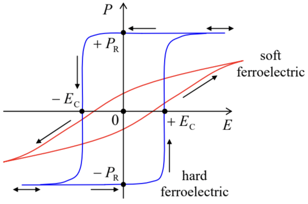 Fig. 3.8. The average polarization of soft and hard ferroelectrics as functions of the applied electric field (schematically).
Depending on the ferroelectric’s material, temperature, and the sample’s geometry (a solid crystal, a ceramic material, or a thin film), the hysteretic loops may be rather different, ranging from a rather smooth form in the so-called soft ferroelectrics (which include most ferroelectric thin films) to an almost rectangular form in hard ferroelectrics – see Fig. 8. In low fields, soft ferroelectrics behave essentially as linear paraelectrics, but with a very high average dielectric constant – see the bottom line of Table 1 for such a classical material as BaTiO3 (which is a soft ferroelectric at temperatures below Tc≈120∘C, and a paraelectric above this critical temperature). On the other hand, the polarization of a hard ferroelectric in the fields below its coercive field remains virtually constant, and the analysis of their electrostatics may be based on the condition P=PR= const – already used in the problem discussed in the end of the previous section.23 This condition is even more applicable to the so-called electrets – synthetic polymers with a spontaneous polarization that remains constant even in very high electric fields.
Some materials exhibit even more complex polarization effects, for example antiferroelectricity, helielectricity, and (practically very valuable) piezoelectricity. Unfortunately, we do not have time for a discussion of these exotic phenomena in this course;24 the main reason I am mentioning them is to emphasize again that the constitutive relation P=P(E) is material-specific rather than fundamental.
However, most insulators, in practicable fields, behave as linear dielectrics, so that the next section will be committed to the discussion of their electrostatics.
Reference
11 In the problem solved at the end of the previous section, the role of such relation was played by the equality P0=const.
12 In older physics literature, the dielectric constant is often denoted by letter εr, while in the electrical engineering publications, its notation is frequently K.
13 The reader may be perplexed by the use of three different but uniquely related parameters (χe, κ≡1+χe, and ε≡κε0) for the description of just one scalar property. Unfortunately, such redundancy is typical for physics, whose
different sub-field communities have different, well-entrenched traditions.
14 In the Gaussian units, χe is defined by the following relation: P=χeE, while ε is defined just as in the SI units, D=εE. Because of that, in the Gaussian units, the constant ε is dimensionless and equals (1+4πχe). As a result, εGaussian =(ε/ε0)SI≡κ, so that (χe)Gaussian =(χe)SI/4π, sometimes creating confusion between the numerical values of the latter parameter – dimensionless in both systems.
15 See, e.g., SM Chapter 2.
16 Realistically, these effects are governed by quantum mechanics, so that the average here should be understood not only in the statistical-mechanical, but also (and mostly) in the quantum-mechanical sense. Because of that, for non-polar atoms, α is typically a very weak function of temperature, at least on the usual scale T∼300 K.
17 See, e.g., SM Secs. 1.4 and 3.1.
18 Such radius is defined by the requirement that the volume of the corresponding sphere, if used in the van-der-Waals equation (see, e. g., SM Sec. 4.1), gives the best fit to the experimental equation of state n=n(P,T).
19 As will be discussed in QM Chapter 6, for a hydrogen atom in its ground state, the low-field polarizability may be calculated analytically: α=(9/2)×4πε0r3B, corresponding to our metallic-ball model with a close value of the effective radius: R=(9/2)1/3rB≈1.65rB≈0.87×10−10 m.
20 Applied to the high-frequency electric field, with κ replaced by the square of the refraction coefficient n at the field’s frequency (see Chapter 7), this formula is known as the Lorenz-Lorentz relation.
21 I am leaving the proof of Eq. (52), using a formula that will be derived in the next section, for the reader's exercise.
22 The Clausius-Mossotti model does not give quantitatively correct results for most ferroelectric materials. For a review of modern approaches to the theory of their polarization, see, e.g., the paper by R. Resta and D. Vanderbilt in the review collection by K. Rabe, C. Ahn, and J.-M. Triscone (eds.), Physics of Ferroelectrics: A Modern Perspective, Springer, 2010.
23 Due to this property, hard ferroelectrics, such as the lead zirconate titanate (PZT) and strontium bismuth tantalite (SBT), with high remnant polarization PR (up to ∼1C/m2), may be used in nonvolatile random-access memories (dubbed either FRAM or FeRAM) – see, e.g., J. Scott, Ferroelectric Memories, Springer, 2000. In a cell of such a memory, binary information is stored in the form of one of two possible directions of spontaneous polarization at E=0 (see Fig. 8). Unfortunately, the time of spontaneous depolarization of ferroelectric thin films is typically well below 10 years – the industrial standard for data retention in nonvolatile memories, and this time may be decreased even more by “fatigue” from the repeated polarization recycling at information recording. Due to these reasons, the industrial production of FRAM is currently just a tiny fraction of the nonvolatile memory market, which is dominated by floating-gate memories – see, e.g., Sec. 4.2 below.
24 For detailed coverage of ferroelectrics, I can recommend the encyclopedic monograph by M. Lines and A. Glass, Principles and Applications of Ferroelectrics and Related Materials, Oxford U. Press, 2001, and the recent review collection edited by K. Rabe et al., that was cited above.