
13.2: Simple Harmonic Motion and Oscillations


- Last updated
- Aug 30, 2024
- Save as PDF
( \newcommand{\kernel}{\mathrm{null}\,}\)
To understand the properties of waves, we start by examining oscillations. An oscillation is a type of repetitive, periodic behavior. This is a fairly wide definition and includes a huge number of systems. In fact, oscillations are an important part of biology, chemistry, economics, ecology, engineering, geology, music and more. The focus for now will be on a specific type of oscillation called simple harmonic oscillation. This is also referred to as simple harmonic motion (SHM).
Even though the 'simple' part of simple harmonic motion requires that we ignore things like friction or air resistance, we can still learn a lot about real-world systems that behave in a similar way. A pendulum swinging back and forth, and a mass attached to a spring are two examples of oscillations that are nearly the same as the simplified system. Before we start, some general definitions are useful.
Oscillation Fundamentals
- Oscillation or Cycle: A process during which the system returns to its initial conditions.
- Amplitude: The maximum displacement from the equilibrium position. This is typically measured in meters and is symbolized by A.
- Period: The length of time the system takes to complete one cycle. This has units of seconds per cycle and is represented by T.
- Frequency: How often the system completes an oscillation. This has units of cycles per second, also called Hertz, written as f. f = 1T
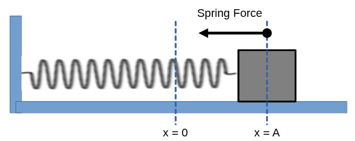
To help build some intuition about oscillating systems imagine a flat, horizontal surface that is frictionless. A stiff spring is attached to a wall, and a block is attached to the other end. The block is in equilibrium, meaning that any forces acting on the block are balanced. The surface supports the block and cancels the effect of gravity. The spring is relaxed, meaning it isn't stretched or compressed. The block is at some distance from the wall. We'll label the position of the block as x, and set x = 0.

Mass-spring system in equilibrium, by Claude Mona, under CC BY NC
Pulling the block to the right would move the block in the positive direction and stretch the spring. We know that spring forces act to try and keep the spring the same length, so stretching the spring to the right means that the spring will pull to the left. If we let go of the block at point x = A, the block will start moving to the left.
Mass-spring system (net spring force), by Claude Mona, under CC BY NC
If we pushed the block to the left, the spring would compress and push to the right. In either case, the spring force acts on the block to try and return the block to the equilibrium position, x = 0. A force that acts this way is called a restoring force, and restoring forces are needed for systems to oscillate. The spring force (restoring force) depends on the properties of the spring and how far the spring has been stretched from equilibrium:
Fspring=−kΔx
Δx is a measure of how far the block has been moved from equilibrium. In the picture above, this would be Δx = A. How far the block is moved from equilibrium is also the definition of amplitude. In this scenario, the amplitude of motion is A.
The 'k' is called the spring constant, and describes the 'stiffness' of the spring. A large k value means that it requires a large force to stretch or compress the spring. The minus sign helps us to remember that the spring is a restoring force that acts to return the block to the equilibrium position. The spring constant typically has units of Newtons per meter.
The stiffer the spring is, the larger the force that acts on the block. Larger forces lead to larger accelerations. Larger accelerations lead to larger speeds. Larger speeds mean shorter times to travel from one point to another. So, we imagine that large k values lead to short periods.
For any particular spring force, the larger the mass of the block, the less it will accelerate. Lower accelerations lead to slower speeds and that should mean longer travel times. Here we see that large mass values lead to longer periods.
Finally, the further the spring is stretched (larger amplitude), the larger the force the spring produces. We see that larger forces lead to larger speeds, but the block also has to travel a greater distance because the spring was stretched further. Larger speeds mean shorter travel times, but greater distances mean longer travel times. At this point, it isn't exactly clear if these effects cancel each other out. Maybe the amplitude has an effect on the period and maybe it doesn't.
Spring 1 requires a force of 54 Newtons to achieve a 14 centimeter stretch. Spring 2 stretches 18 centimeters when a 62 Newton force is applied. Which one stretches the furthest when a 9 Newton force is applied to it?
Solution
The spring constant provides information about the 'stretchiness' of the spring. Spring 1: k1 = 54Newtons0.14meters = 385.7 Nm. Spring 2: k2 = 62Newtons0.18meters = 344.4 Nm.
Since spring 2 has the lower spring constant, it will stretch more for any applied force. You could also take the reciprocal of k and calculate the amount of stretch per Newton of force applied. For spring 1, this is 2.59 millimeters per Newton and spring 2 stretches 2.9 millimeters per Newton.